DDE too stiff? radau method required? #198
Description
Hi Everyone,
The following is a question I recently asked on Julia Discourse (https://discourse.julialang.org/t/dde-too-stiff-required-tolerances-are-too-slow/52259) about an issue solving a very stiff set of DDEs. I found some improvement by tweaking the solver options (e.g., specifying dtstops = initTauU and dtmax = 0.1 ), but Chris thought this might require a radau method so I'm opening this issue in case someone wants to tackle it and use this as a benchmark problem. Any help is greatly appreciated!
Original question:
I have a system of DDEs that model host-parasite dynamics in a seasonal environment and I am having some issues because (I think) the equations are so stiff. Basically, when the number of hosts S is too high (> about 500) I have to lower the solver tolerances so much that it becomes prohibitively slow (I need S up to about a 4e6). I believe the low tolerances are required because u[1] decreases to zero so rapidly when S is high that the history function (W_past) just returns zero, which makes matU = 0.0 and therefore u[3] stays at 0.0 (i.e., no infective larvae develop). It may be the case that I just have to use low tolerances and run the simulation for hours and hours, but if anyone has any suggestions to make this work without having to lower the tolerances too much I would be very grateful. I tried several different stiff solvers (Rosenbrock23, Rodas3,4,4P&5, etc.) but without any great success. Maybe some way of adjusting the step size or addressing the discontinuity is possible? Any other general performance tips are also appreciated.
Here is a stripped down MWE:
using QuadGK, Roots, DelayDiffEq, Plots

#parameters

const Temp0K = 15+273.15;
const k = 8.62 * 10^(-5);
const S = 100.0         #Host density

const mu_W_a = 0.0186;
const mu_W_E = 0.87;
const mu_W_EH = 5.0*mu_W_E;
const mu_W_TH = 289.65;
const Phi_a = 0.024;
const Phi_E = 0.46;

const mu_U_a = 0.0001;
const mu_U_E = 0.87;
const mu_U_EH = 5.0*mu_U_E;
const mu_U_TH = 289.65;

const tauU_a = 25.1;
const tauU_E = 0.87;
const tauU_EL = 5.0*tauU_E;
const tauU_TL = 282.0218;

#Development function

function g_U(T)
    tmp = 1 / max(TempKstop, T)
    1 / (tauU_a * exp((tauU_E/k) * (tmp - (1 / Temp0K))) *
      (1 + exp((tauU_EL / k) * (tmp - (1 / tauU_TL)))))
end

function mu_W(T)
  tmp = 1 / max(TempKstop, T)
  mu_W_a * exp((-mu_W_E/k)*((tmp)-(1/Temp0K))) * (1 + exp((mu_W_EH/k)*((-tmp)+(1/mu_W_TH)))); #L1 mort
end

function mu_U(T)
  tmp = 1 / max(TempKstop, T)
  mu_U = mu_U_a * exp((-mu_U_E/k)*((tmp)-(1/Temp0K))) * (1 + exp((mu_U_EH/k)*((-tmp)+(1/mu_U_TH)))); #U mort
end

function Phi(T)
  tmp = 1 / max(TempKstop, T)
  Phi = Phi_a * exp((-Phi_E/k)*((tmp)-(1/Temp0K))); #W penetration into slugs
end


function Re_MWE(du,u,h,p,t)
  #State variables
   W = u[1]; U = u[2]; I = u[3]; DU1 = u[4]; tauU = u[5];

   # History calculations
   ucache = h(p, t - tauU)
   W_past = ucache[1]
   U_past = ucache[2]

   # Compute temperature
   T = Temp(t)
   T_past = Temp(t - tauU)

   # Preliminary calculations
   gU_ratio = g_U(T) / g_U(T_past)
   matW = Phi(T) * S * W #Maturation rate of W
   matU = Phi(T_past) * S * W_past * DU1 * gU_ratio

 #Model

   du[1] =  - mu_W(T) * W - matW                        #W) Free-living L1s
   du[2] = matW - U * mu_U(T) - matU                    #U) Uninfective larvae
   du[3] = matU                                         #I) Infective larvae
   du[4] = DU1 * (mu_U(T_past) * U_past / S * gU_ratio - mu_U(T) * U / S) #Survival probability through delay period
   du[5] = 1 - gU_ratio                                 #tauU) Change in delay duration
 nothing
 end

 #Setup simualation

 #Initial conditions and history
   const InitW = 1.0;
   const InitU = 0.0;
   const InitI = 0.0;

function DySimulate1(alg, tstart, tfin, tol)
        gint(u) = quadgk(g_U ∘ Temp, tstart - u, tstart)[1]
        initTauU = [fzero(u -> gint(u) - p, [0.001, 5000]) for p in [1.0]][1] #Initial lag for each day (where guadgk = 1.0)
        mUint = exp(-(quadgk(mu_U ∘ Temp, tstart-initTauU, tstart)[1]))

        DUinit = mUint
        DUhist = DUinit
        u0 = [InitW, InitU, InitI, DUinit,initTauU]
        h(p,t) = [0.0, 0.0, 0.0, DUhist, initTauU]
        tspan = (tstart, tfin+tstart)

        # Declare dependent lags
        probDynSea = DDEProblem(Re_MWE, u0, h, tspan;
                              dependent_lags = ((u, p, t) -> u[5],))

      solDynSimpSea = solve(probDynSea,alg;  isoutofdomain=(u,p,t) -> any(x -> x < 0.0, u), abstol = tol, reltol = tol)#, save_idxs = 3)
      #solDynSimpSea = solve(probDynSea,alg; dtmax = 0.1, tstops = [initTauU], isoutofdomain=(u,p,t) -> any(x -> x < 0.0, u), abstol = tol, reltol = tol)#, save_idxs = 3)

end

alg = MethodOfSteps(Rosenbrock23())
# alg = MethodOfSteps(Rosenbrock32())
# alg = MethodOfSteps(Rodas4P())
# alg = MethodOfSteps(Rodas4())
# alg = MethodOfSteps(Rodas5())
# alg = MethodOfSteps(TRBDF2())
# alg = MethodOfSteps(KenCarp4())

#Temperature function
const c_K = 263.0; #Mean annual temperature (Kelvins)
const d_K = 0.66478 * c_K + -153.14
const t0 = -1.6962 * c_K +551.43
const TempKstop = 273.15-0.0
Temp(t) = c_K + d_K * sin((t-t0)*2*pi/365);

MWEanswer = DySimulate1(alg,1.0,365.0*2, 1e-4)
p = plot(MWEanswer, vars = (0,[3]))
# scatter!(p,MWEanswer.t, MWEanswer.u)
# p
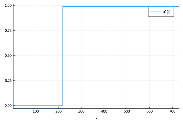
When both the solver tolerances are tol = 1e-4 and S = 100.0 then I get this:
But when tol = 1e-4 and S = 700.0 I get this:
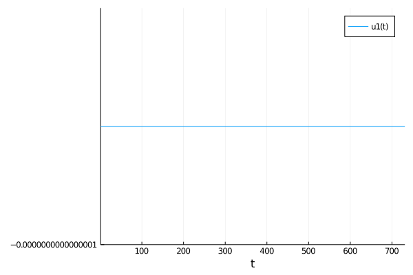
Once I lower the tolerances to tol = 1e-6 with S = 700.0 it works again, but is much much slower and requires larger maxiters. However, with my full model this approach is just too slow, I end up needing to go at least 1e-10 to get anything other than the flat line. I hope I've explained my problem clearly. Thanks.