You signed in with another tab or window. Reload to refresh your session.You signed out in another tab or window. Reload to refresh your session.You switched accounts on another tab or window. Reload to refresh your session.Dismiss alert
# Ruby Numo::Gnuplot Demo in single page
Translated from [Gnuplot Demo](http://gnuplot.sourceforge.net/demo_4.6/)
* [GitHub](https://github.com/ruby-numo/numo-gnuplot-demo/tree/master/gnuplot)
## simple functions
[Original Demo](http://gnuplot.sourceforge.net/demo_4.6/simple.html)
### 1
```ruby
# # Requires data files "[123].dat" from this directory,
# # so change current working directory to this directory before running.
# # gnuplot> set term
# # gnuplot> load 'simple.dem'
# #
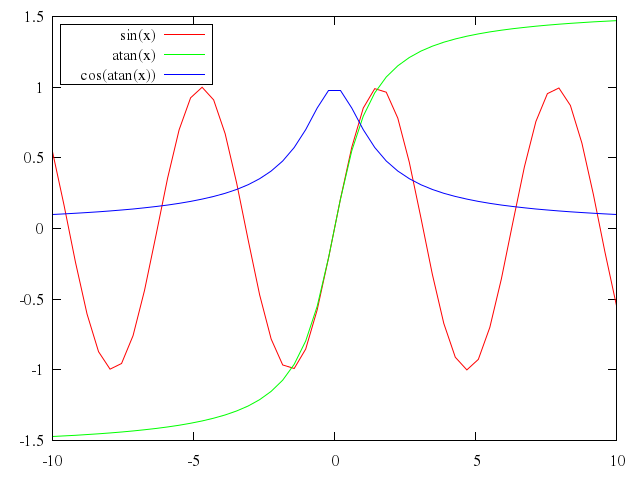
# set key left box
# set samples 50
# plot [-10:10] sin(x),atan(x),cos(atan(x))
Numo.gnuplot do
set :key, :left, :box
set samples:50
plot -10..10,
"sin(x)",
"atan(x)",
"cos(atan(x))"
end
```
### 2
```ruby
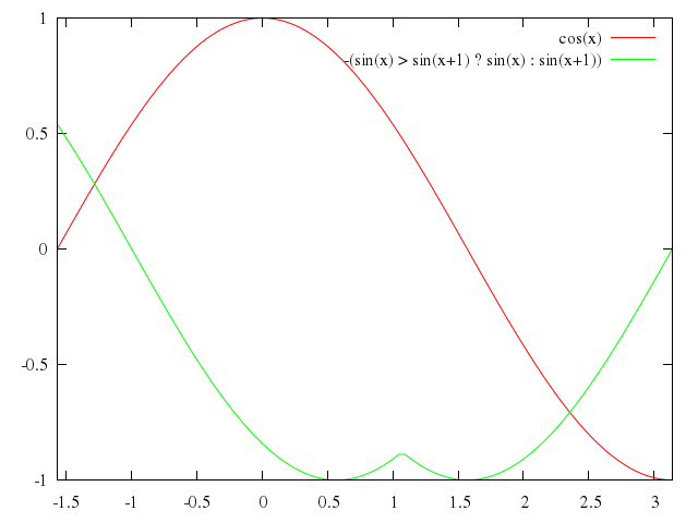
# set key right nobox
# set samples 100
# plot [-pi/2:pi] cos(x),-(sin(x) > sin(x+1) ? sin(x) : sin(x+1))
Numo.gnuplot do
set :key, :right, :nobox
set samples:100
plot "[-pi/2:pi]",
"cos(x)",
"-(sin(x) > sin(x+1) ? sin(x) : sin(x+1))"
end
```
### 3
```ruby
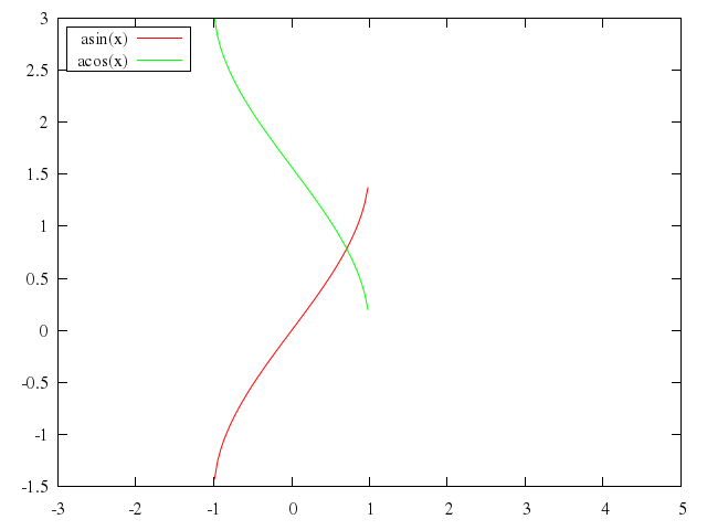
# set key left box
# set samples 200
# plot [-3:5] asin(x),acos(x)
Numo.gnuplot do
set :key, :left, :box
set samples:200
plot -3..5,
"asin(x)",
"acos(x)"
end
```
### 4
```ruby
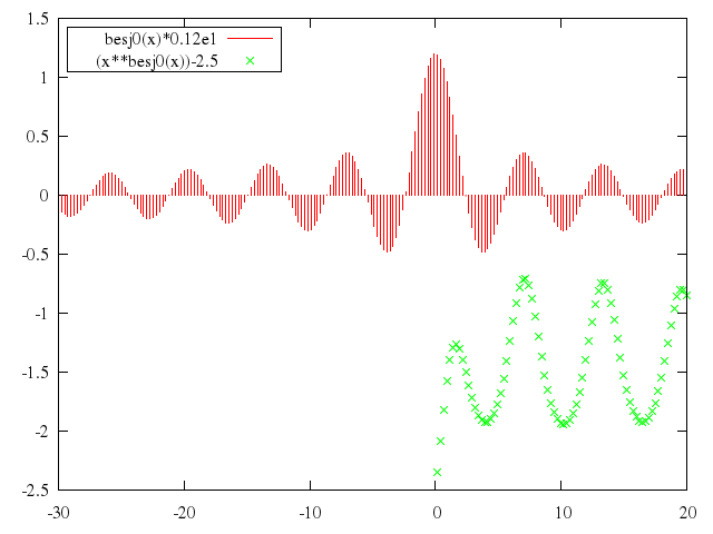
# plot [-30:20] besj0(x)*0.12e1 with impulses, (x**besj0(x))-2.5 with points
Numo.gnuplot do
plot -30..20,
["besj0(x)*0.12e1", with:"impulses"],
["(x**besj0(x))-2.5", with:"points"]
end
```
### 5
```ruby
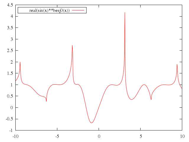
# set samples 400
# plot [-10:10] real(sin(x)**besj0(x))
Numo.gnuplot do
set samples:400
plot -10..10,
"real(sin(x)**besj0(x))"
end
```
### 6
```ruby
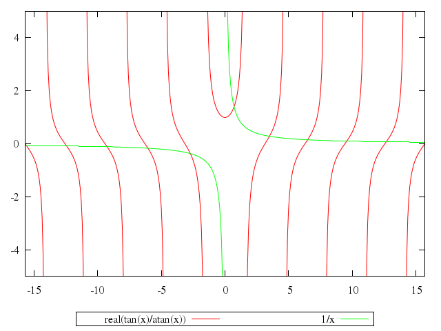
# set key bmargin center horizontal
# plot [-5*pi:5*pi] [-5:5] real(tan(x)/atan(x)), 1/x
Numo.gnuplot do
set :key, :bmargin, :center, :horizontal
plot "[-5*pi:5*pi]", -5..5,
"real(tan(x)/atan(x))",
"1/x"
end
```
### 7
```ruby
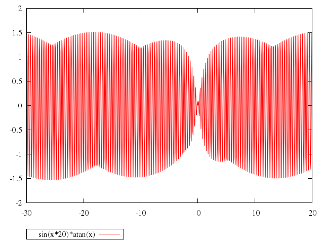
# set key left box
# set autoscale
# set samples 800
# plot [-30:20] sin(x*20)*atan(x)
Numo.gnuplot do
set :key, :left, :box
set :autoscale
set samples:800
plot -30..20,
"sin(x*20)*atan(x)"
end
```
### 8
```ruby
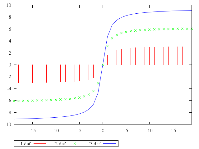
# plot [-19:19] '1.dat' with impulses, '2.dat', '3.dat' with lines
Numo.gnuplot do
plot -19..19,
["'1.dat'", with:"impulses"],
"'2.dat'",
["'3.dat'", with:"lines"]
end
```
## filled curves
[Original Demo](http://gnuplot.sourceforge.net/demo_4.6/fillcrvs.html)
### 1
```ruby
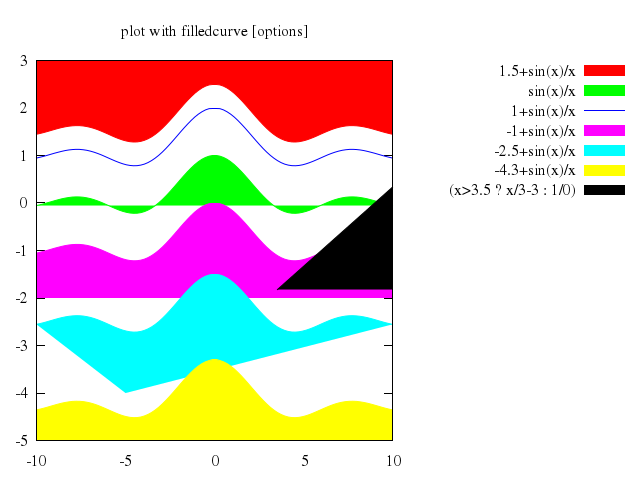
# ### Demo for 'with filledcurves'
#
# reset
#
# set title
# set key outside
# set title "plot with filledcurve [options]"
# plot [-10:10] [-5:3] \
# 1.5+sin(x)/x with filledcurve x2, \
# sin(x)/x with filledcurve, \
# 1+sin(x)/x with lines, \
# -1+sin(x)/x with filledcurve y1=-2, \
# -2.5+sin(x)/x with filledcurve xy=-5,-4., \
# -4.3+sin(x)/x with filledcurve x1, \
# (x>3.5 ? x/3-3 : 1/0) with filledcurve y2
Numo.gnuplot do
reset
set :title
set :key, :outside
set title:"plot with filledcurve [options]"
plot -10..10, -5..3,
["1.5+sin(x)/x", with:'filledcurve x2'],
["sin(x)/x", with:"filledcurve"],
["1+sin(x)/x", with:"lines"],
["-1+sin(x)/x", with:'filledcurve y1=-2'],
["-2.5+sin(x)/x", with:'filledcurve xy=-5,-4.'],
["-4.3+sin(x)/x", with:'filledcurve x1'],
["(x>3.5 ? x/3-3 : 1/0)", with:'filledcurve y2']
end
```
### 2
```ruby
# set key on
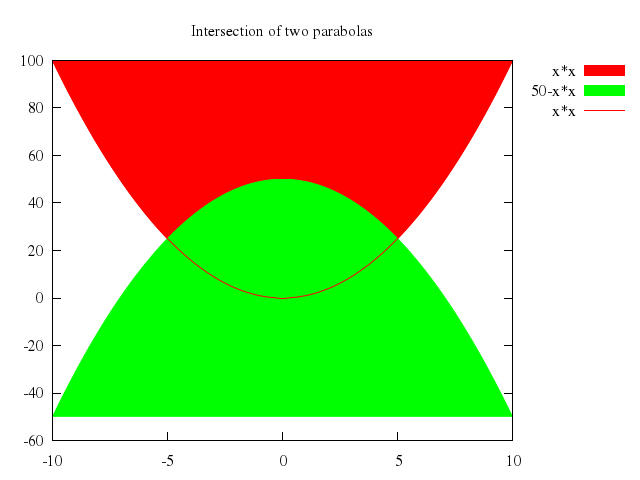
# set title "Intersection of two parabolas"
# plot x*x with filledcurves, 50-x*x with filledcurves, x*x with line lt 1
Numo.gnuplot do
set :key, :on
set title:"Intersection of two parabolas"
plot ["x*x", with:"filledcurves"],
["50-x*x", with:"filledcurves"],
["x*x", with:"line", lt:1]
end
```
### 3
```ruby
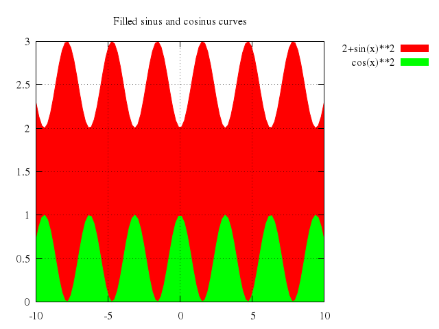
# set grid front
# set title "Filled sinus and cosinus curves"
# plot 2+sin(x)**2 with filledcurve x1, cos(x)**2 with filledcurve x1
Numo.gnuplot do
set :grid, :front
set title:"Filled sinus and cosinus curves"
plot ["2+sin(x)**2", with:'filledcurve x1'],
["cos(x)**2", with:'filledcurve x1']
end
```
### 4
```ruby
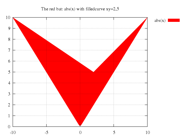
# set title "The red bat: abs(x) with filledcurve xy=2,5"
# plot abs(x) with filledcurve xy=2,5
Numo.gnuplot do
set title:"The red bat: abs(x) with filledcurve xy=2,5"
plot "abs(x)", with:'filledcurve xy=2,5'
end
```
### 5
```ruby
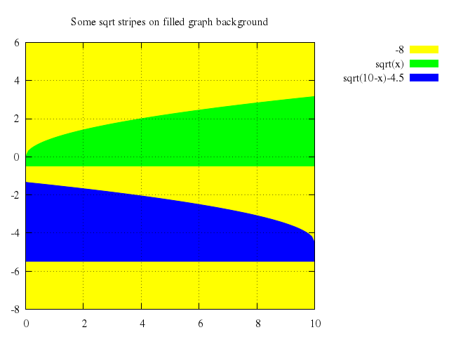
# set title "Some sqrt stripes on filled graph background"
# plot [0:10] [-8:6] \
# -8 with filledcurve x2 lt 15, \
# sqrt(x) with filledcurves y1=-0.5, \
# sqrt(10-x)-4.5 with filledcurves y1=-5.5
Numo.gnuplot do
set title:"Some sqrt stripes on filled graph background"
plot 0..10, -8..6,
["-8", with:'filledcurve x2', lt:15],
["sqrt(x)", with:'filledcurves y1=-0.5'],
["sqrt(10-x)-4.5", with:'filledcurves y1=-5.5']
end
```
### 6
```ruby
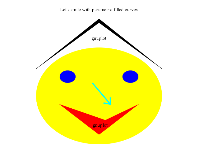
# reset
# set title "Let's smile with parametric filled curves"
# set size square
# set key off
# unset border
# unset xtics
# unset ytics
# set grid
# set arrow 1 from -0.1,0.26 to 0.18,-0.17 front size 0.1,40 lt 5 lw 4
# set label 1 "gnuplot" at 0,1.2 center front
# set label 2 "gnuplot" at 0.02,-0.6 center front
# set parametric
# set xrange [-1:1]
# set yrange [-1:1.6]
# plot [t=-pi:pi] \
# sin(t),cos(t) with filledcurve xy=0,0 lt 15, \
# sin(t)/8-0.5,cos(t)/8+0.4 with filledcurve lt 3, \
# sin(t)/8+0.5,cos(t)/8+0.4 with filledcurve lt 3, \
# t/5,abs(t/5)-0.8 with filledcurve xy=0.1,-0.5 lt 1, \
# t/3,1.52-abs(t/pi) with filledcurve xy=0,1.8 lt -1
Numo.gnuplot do
reset
set title:"Let's smile with parametric filled curves"
set size:"square"
set :key, :off
unset :border
unset :xtics
unset :ytics
set :grid
set :arrow, 1, from:[-0.1,0.26], to:[0.18,-0.17], front:true, size:[0.1,40], lt:5, lw:4
set :label, 1, "gnuplot", at:[0,1.2], center:true, front:true
set :label, 2, "gnuplot", at:[0.02,-0.6], center:true, front:true
set :parametric
set xrange:-1..1
set yrange:-1..1.6
plot "[t=-pi:pi]",
"sin(t)",
["cos(t)", with:'filledcurve xy=0,0', lt:15],
"sin(t)/8-0.5",
["cos(t)/8+0.4", with:"filledcurve", lt:3],
"sin(t)/8+0.5",
["cos(t)/8+0.4", with:"filledcurve", lt:3],
"t/5",
["abs(t/5)-0.8", with:'filledcurve xy=0.1,-0.5', lt:1],
"t/3",
["1.52-abs(t/pi)", with:'filledcurve xy=0,1.8', lt:-1]
end
```
### 7
```ruby
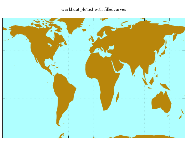
# reset
#
# set title "world.dat plotted with filledcurves"
# set format x ""
# set format y ""
# set grid layerdefault linewidth 0.5
# set object 1 rect from graph 0, 0 to graph 1, 1 behind fc rgb "#afffff" fillstyle solid 1.00 border -1
# set xrange [ -180.000 : 180.000 ]
# set yrange [ -70.0000 : 80.0000 ]
# set lmargin 1
# plot 'world.dat' with filledcurve notitle fs solid 1.0 lc rgb 'dark-goldenrod'
Numo.gnuplot do
reset
set title:"world.dat plotted with filledcurves"
set format_x:""
set format_y:""
set :grid, "layerdefault", linewidth:0.5
set :object, 1, "rect", from_graph:[0,0], to_graph:[1,1], behind:true, fc_rgb:"#afffff", fillstyle_solid:1.00, border:-1
set xrange:-180.000..180.000
set yrange:-70.0000..80.0000
set lmargin:1
plot "'world.dat'", with:"filledcurve", notitle:true, fs_solid:1.0, lc_rgb:'dark-goldenrod'
end
```
## fill between curves
[Original Demo](http://gnuplot.sourceforge.net/demo_4.6/fillbetween.html)
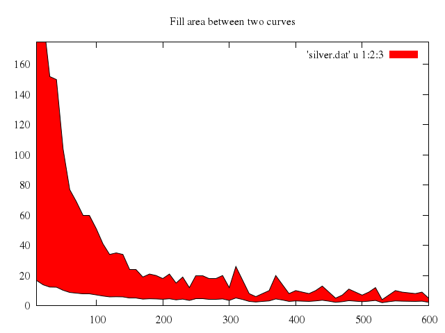
### 1
```ruby
# # Demonstrate filling the area between two curves
# # and also the application of fillstyle to filled curves.
# # Ethan Merritt
# # June 2004
# #
# set title "Fill area between two curves"
# set style data lines
# set xrange [10:*]
# set yrange [0:175]
# plot 'silver.dat' u 1:2:3 w filledcu, \
# '' u 1:2 lt -1 notitle, '' u 1:3 lt -1 notitle
Numo.gnuplot do
set title:"Fill area between two curves"
set :style, :data, :lines
set xrange:"[10:*]"
set yrange:0..175
plot ["'silver.dat'", u:[1,2,3], w:"filledcu"],
["''", u:[1,2], lt:-1, notitle:true],
["''", u:[1,3], lt:-1, notitle:true]
end
```
### 2
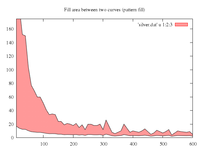
```ruby
# set style fill pattern 2
# set title "Fill area between two curves (pattern fill)"
# replot
Numo.gnuplot do
set :style, :fill, pattern:2
set title:"Fill area between two curves (pattern fill)"
replot
end
```
### 3
```ruby
# set title "Fill area between two curves (above/below)"
# set style fill solid 1.0 noborder
# set xrange [250:500]
# set auto y
# plot 'silver.dat' u 1:2:($3+$1/50.) w filledcurves above title 'Above', \
# '' u 1:2:($3+$1/50.) w filledcurves below title 'Below', \
# '' u 1:2 lt -1 lw 2 title 'curve 1', \
# '' u 1:($3+$1/50.) lt 3 lw 2 title 'curve 2'
Numo.gnuplot do
set title:"Fill area between two curves (above/below)"
set :style, fill_solid:1.0, noborder:true
set xrange:250..500
set auto:"y"
plot ["'silver.dat'", u:'1:2:($3+$1/50.)', w:'filledcurves above', title:'Above'],
["''", u:'1:2:($3+$1/50.)', w:'filledcurves below', title:'Below'],
["''", u:[1,2], lt:-1, lw:2, title:'curve 1'],
["''", u:'1:($3+$1/50.)', lt:3, lw:2, title:'curve 2']
end
```

## candlesticks
[Original Demo](http://gnuplot.sourceforge.net/demo_4.6/candlesticks.html)
### 1
```ruby
# reset
# #
# set xrange [0:11]
# set yrange [0:10]
# #
# set title "candlesticks with open boxes (default)"
# plot 'candlesticks.dat' using 1:3:2:6:5 with candlesticks
Numo.gnuplot do
reset
set xrange:0..11
set yrange:0..10
set title:"candlesticks with open boxes (default)"
plot "'candlesticks.dat'", using:[1,3,2,6,5], with:"candlesticks"
end
```

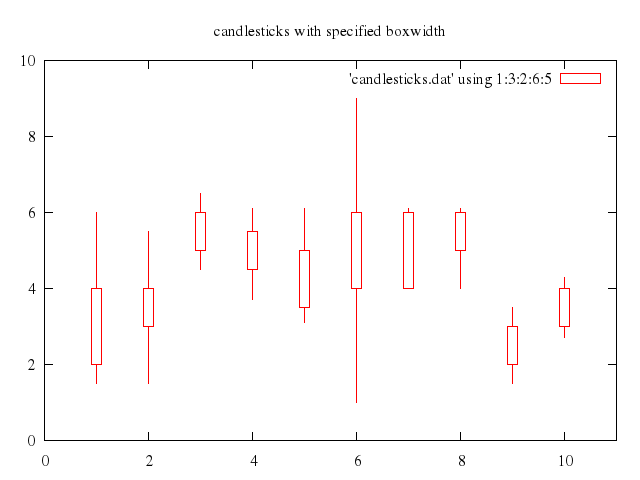
### 2
```ruby
# set title "candlesticks with specified boxwidth"
# set boxwidth 0.2
# replot
Numo.gnuplot do
set title:"candlesticks with specified boxwidth"
set boxwidth:0.2
replot
end
```
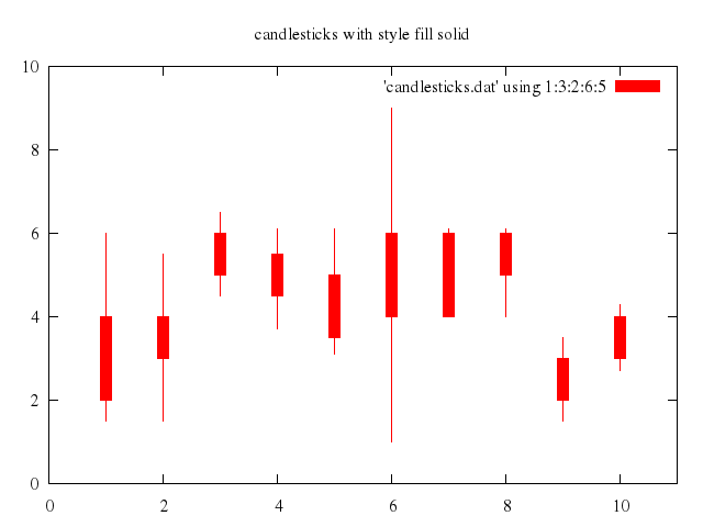
### 3
```ruby
# set title "candlesticks with style fill solid"
# set style fill solid
# set boxwidth 0.2
# replot
Numo.gnuplot do
set title:"candlesticks with style fill solid"
set :style, :fill_solid
set boxwidth:0.2
replot
end
```
### 4
```ruby
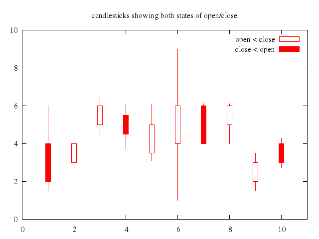
# set title "candlesticks showing both states of open/close"
# set style fill empty
# set boxwidth 0.2
# plot 'candlesticks.dat' using 1:(int($0)%3?$3:$5):2:6:(int($0)%3?$5:$3) with candlesticks title "open < close", \
# NaN with boxes lt 1 fs solid 1 title "close < open"
Numo.gnuplot do
set title:"candlesticks showing both states of open/close"
set :style, :fill, :empty
set boxwidth:0.2
plot ["'candlesticks.dat'", using:'1:(int($0)%3?$3:$5):2:6:(int($0)%3?$5:$3)', with:"candlesticks", title:"open < close"],
["NaN", with:"boxes", lt:1, fs_solid:1, title:"close < open"]
end
```
### 5
```ruby
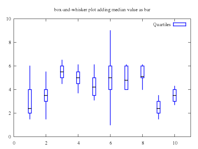
# set title "box-and-whisker plot adding median value as bar"
# set style fill empty
# plot 'candlesticks.dat' using 1:3:2:6:5 with candlesticks lt 3 lw 2 title 'Quartiles', \
# '' using 1:4:4:4:4 with candlesticks lt -1 lw 2 notitle
Numo.gnuplot do
set title:"box-and-whisker plot adding median value as bar"
set :style, :fill, :empty
plot ["'candlesticks.dat'", using:[1,3,2,6,5], with:"candlesticks", lt:3, lw:2, title:'Quartiles'],
["''", using:[1,4,4,4,4], with:"candlesticks", lt:-1, lw:2, notitle:true]
end
```
### 6
```ruby
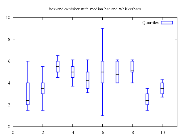
# set title "box-and-whisker with median bar and whiskerbars"
# plot 'candlesticks.dat' using 1:3:2:6:5 with candlesticks lt 3 lw 2 title 'Quartiles' whiskerbars, \
# '' using 1:4:4:4:4 with candlesticks lt -1 lw 2 notitle
Numo.gnuplot do
set title:"box-and-whisker with median bar and whiskerbars"
plot ["'candlesticks.dat'", using:[1,3,2,6,5], with:"candlesticks", lt:3, lw:2, title:'Quartiles', whiskerbars:true],
["''", using:[1,4,4,4,4], with:"candlesticks", lt:-1, lw:2, notitle:true]
end
```
## error bars
[Original Demo](http://gnuplot.sourceforge.net/demo_4.6/mgr.html)
### 1
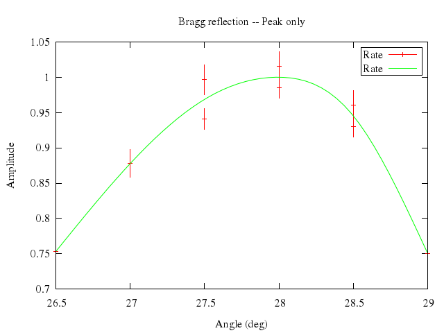
```ruby
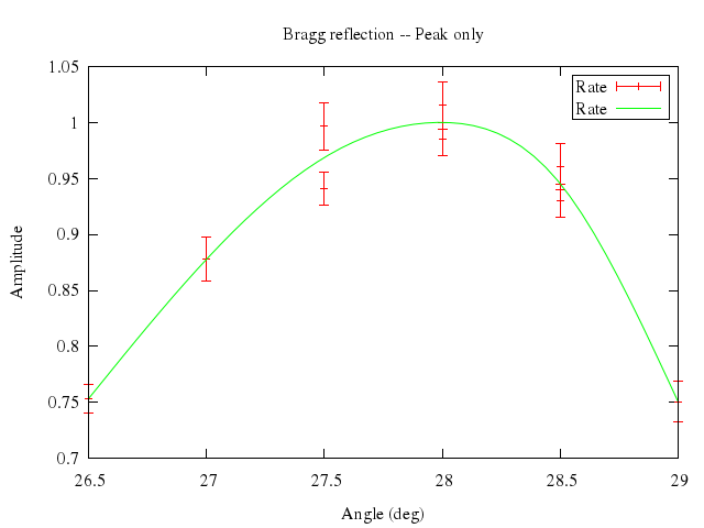
# print "Watch some cubic splines"
# set samples 50
# set xlabel "Angle (deg)"
# set ylabel "Amplitude"
# set key box
# set title "Bragg reflection -- Peak only"
# plot "big_peak.dat" title "Rate" with errorbars, \
# "" smooth csplines t "Rate"
Numo.gnuplot do
set samples:50
set xlabel:"Angle (deg)"
set ylabel:"Amplitude"
set :key, :box
set title:"Bragg reflection -- Peak only"
plot ["\"big_peak.dat\"", title:"Rate", with:"errorbars"],
["\"\"", smooth:"csplines", t:"Rate"]
end
```
### 2
```ruby
# set bars small
# replot
Numo.gnuplot do
set bars:"small"
replot
end
```
### 3
```ruby
# set bars large
# #
# set samples 300
# set xlabel "Time (sec)"
# set ylabel "Rate"
# set title "Ag 108 decay data"
# plot "silver.dat" t "experimental" w errorb, \
# "" smooth csplines t "cubic smooth"
Numo.gnuplot do
set bars:"large"
set samples:300
set xlabel:"Time (sec)"
set ylabel:"Rate"
set title:"Ag 108 decay data"
plot ["\"silver.dat\"", t:"experimental", w:"errorb"],
["\"\"", smooth:"csplines", t:"cubic smooth"]
end
```

### 4
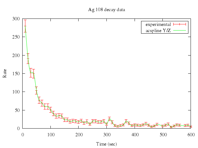
```ruby
# # error is column 3; weight larger errors less
# # start with rel error = 1/($3/$2)
# S=1
# plot "silver.dat" t "experimental" w errorb,\
# "" u 1:2:(S*$2/$3) smooth acsplines t "acspline Y/Z"
Numo.gnuplot do
run "S=1"
plot ["\"silver.dat\"", t:"experimental", w:"errorb"],
["\"\"", u:'1:2:(S*$2/$3)', smooth:"acsplines", t:"acspline Y/Z"]
end
```
### 5
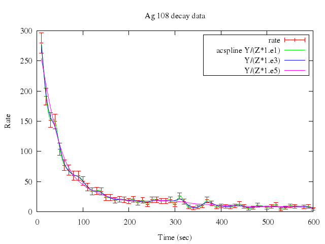
```ruby
# plot "silver.dat" t "rate" w errorb,\
# "" u 1:2:($2/($3*1.e1)) sm acs t "acspline Y/(Z*1.e1)",\
# "" u 1:2:($2/($3*1.e3)) sm acs t " Y/(Z*1.e3)",\
# "" u 1:2:($2/($3*1.e5)) sm acs t " Y/(Z*1.e5)"
Numo.gnuplot do
plot ["\"silver.dat\"", t:"rate", w:"errorb"],
["\"\"", u:'1:2:($2/($3*1.e1))', sm:"acs", t:"acspline Y/(Z*1.e1)"],
["\"\"", u:'1:2:($2/($3*1.e3))', sm:"acs", t:" Y/(Z*1.e3)"],
["\"\"", u:'1:2:($2/($3*1.e5))', sm:"acs", t:" Y/(Z*1.e5)"]
end
```
### 6
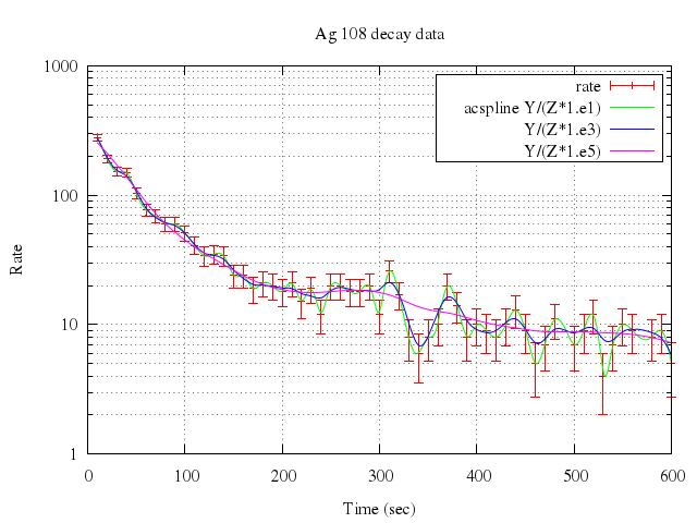
```ruby
# set logscale y
# set grid x y mx my
# replot
Numo.gnuplot do
set logscale:"y"
set :grid, "x y mx my"
replot
end
```
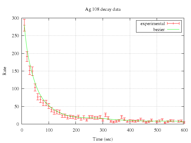
### 7
```ruby
# unset logscale y
# plot "silver.dat" t "experimental" w errorb,\
# "" smooth sbezier t "bezier"
Numo.gnuplot do
unset logscale:"y"
plot ["\"silver.dat\"", t:"experimental", w:"errorb"],
["\"\"", smooth:"sbezier", t:"bezier"]
end
```
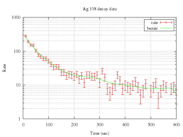
### 8
```ruby
# set logscale y
# plot "silver.dat" t "rate" w errorb, \
# "" smooth sbezier t "bezier"
Numo.gnuplot do
set logscale:"y"
plot ["\"silver.dat\"", t:"rate", w:"errorb"],
["\"\"", smooth:"sbezier", t:"bezier"]
end
```
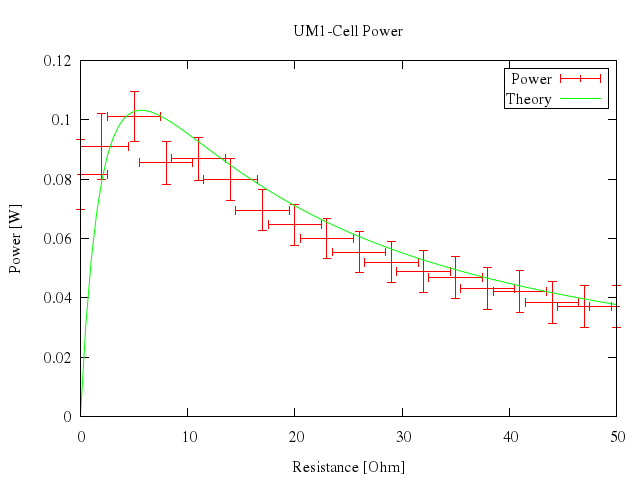
### 9
```ruby
# set samples 100
# unset logscale
# unset grid
# set xlabel "Resistance [Ohm]"
# set ylabel "Power [W]"
# set title "UM1-Cell Power"
# n(x)=1.53**2*x/(5.67+x)**2
# plot [0:50] "battery.dat" t "Power" with xyerrorbars, n(x) t "Theory" w lines
Numo.gnuplot do
set samples:100
unset :logscale
unset :grid
set xlabel:"Resistance [Ohm]"
set ylabel:"Power [W]"
set title:"UM1-Cell Power"
run "n(x)=1.53**2*x/(5.67+x)**2"
plot 0..50,
["\"battery.dat\"", t:"Power", with:"xyerrorbars"],
["n(x)", t:"Theory", w:"lines"]
end
```
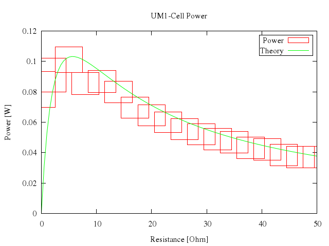
### 10
```ruby
# plot [0:50] "battery.dat" t "Power" with boxxy, n(x) t "Theory" w lines
Numo.gnuplot do
plot 0..50,
["\"battery.dat\"", t:"Power", with:"boxxy"],
["n(x)", t:"Theory", w:"lines"]
end
```
### 11
```ruby
# plot [0:50] "battery.dat" u 1:2:3 t "Power" w xerr, n(x) t "Theory" w lines
Numo.gnuplot do
plot 0..50,
["\"battery.dat\"", u:[1,2,3], t:"Power", w:"xerr"],
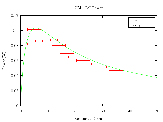
["n(x)", t:"Theory", w:"lines"]
end
```
### 12
```ruby
# plot [0:50] "battery.dat" u 1:2:4 t "Power" w yerr, n(x) t "Theory" w lines
Numo.gnuplot do
plot 0..50,
["\"battery.dat\"", u:[1,2,4], t:"Power", w:"yerr"],
["n(x)", t:"Theory", w:"lines"]
end
```

### 13
```ruby
# set logscale y
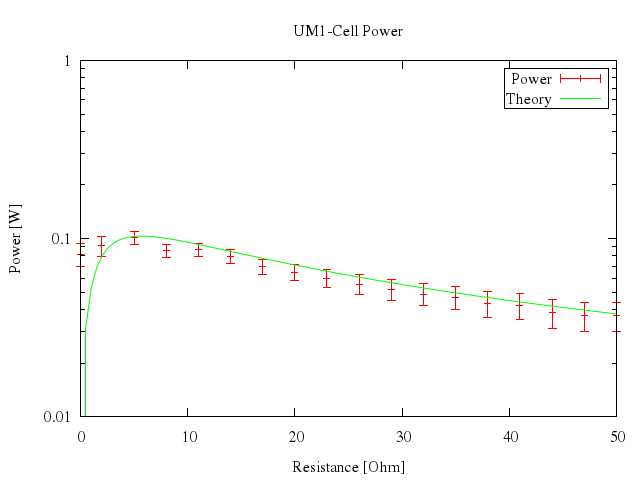
# plot [0:50] "battery.dat" u 1:2:4 t "Power" w yerr, n(x) t "Theory" w lines
Numo.gnuplot do
set logscale:"y"
plot 0..50,
["\"battery.dat\"", u:[1,2,4], t:"Power", w:"yerr"],
["n(x)", t:"Theory", w:"lines"]
end
```
### 14
```ruby
# set logscale xy
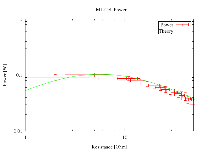
# plot [1:50] "battery.dat" t "Power" w xyerr, n(x) t "Theory" w lines
Numo.gnuplot do
set logscale:"xy"
plot 1..50,
["\"battery.dat\"", t:"Power", w:"xyerr"],
["n(x)", t:"Theory", w:"lines"]
end
```
### 15
```ruby
# unset logscale
# set bars small
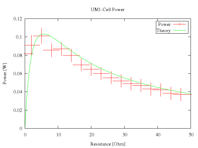
# plot [0:50] "battery.dat" t "Power" with xyerrorbars, n(x) t "Theory" w lines
Numo.gnuplot do
unset :logscale
set bars:"small"
plot 0..50,
["\"battery.dat\"", t:"Power", with:"xyerrorbars"],
["n(x)", t:"Theory", w:"lines"]
end
```
### 16
```ruby
# plot [0:50] "battery.dat" u 1:2:3 t "Power" w xerr, n(x) t "Theory" w lines
Numo.gnuplot do
plot 0..50,
["\"battery.dat\"", u:[1,2,3], t:"Power", w:"xerr"],
["n(x)", t:"Theory", w:"lines"]
end
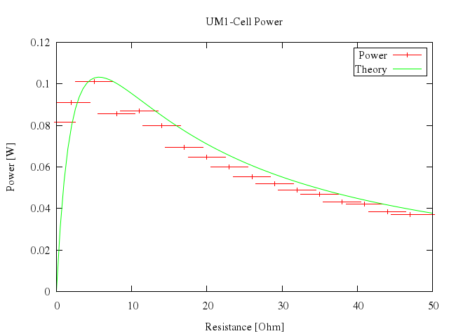
```
### 17
```ruby
# plot [0:50] "battery.dat" u 1:2:4 t "Power" w yerr, n(x) t "Theory" w lines
Numo.gnuplot do
plot 0..50,
["\"battery.dat\"", u:[1,2,4], t:"Power", w:"yerr"],
["n(x)", t:"Theory", w:"lines"]
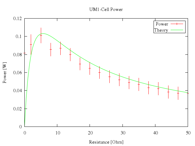
end
```
## histograms
[Original Demo](http://gnuplot.sourceforge.net/demo_4.6/histograms.html)
### 1
```ruby
# # Example of using histogram modes
# #
# reset
# set title "US immigration from Europe by decade"
# set datafile missing "-"
# set xtics nomirror rotate by -45
# set key noenhanced
# #
# # First plot using linespoints
# set style data linespoints
# plot 'immigration.dat' using 2:xtic(1) title columnheader(2), \
# for [i=3:22] '' using i title columnheader(i)
Numo.gnuplot do
reset
set title:"US immigration from Europe by decade"
set :datafile, :missing, "-"
set :xtics, :nomirror, rotate_by:-45
set :key, :noenhanced
set :style, :data, :linespoints
plot ["'immigration.dat'", using:'2:xtic(1)', title_nq:'columnheader(2)'],
"for [i=3:22] '' using i title columnheader(i)"
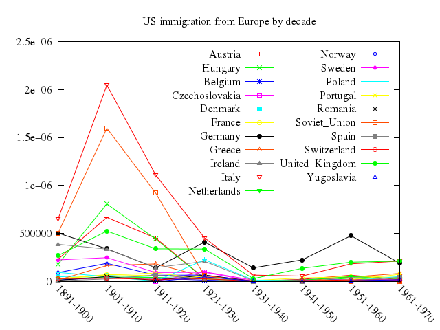
end
```
### 2
```ruby
# set title "US immigration from Northern Europe\nPlot selected data columns as histogram of clustered boxes"
# set auto x
# set yrange [0:300000]
# set style data histogram
# set style histogram cluster gap 1
# set style fill solid border -1
# set boxwidth 0.9
# set xtic rotate by -45 scale 0
# #set bmargin 10
# plot 'immigration.dat' using 6:xtic(1) ti col, '' u 12 ti col, '' u 13 ti col, '' u 14 ti col
Numo.gnuplot do
set title:"US immigration from Northern Europe\nPlot selected data columns as histogram of clustered boxes"
set auto:"x"
set yrange:0..300000
set :style, :data, :histogram
set :style, :histogram, :cluster, gap:1
set :style, :fill_solid, border:-1
set boxwidth:0.9
set :xtic, :rotate, by:-45, scale:0
plot ["'immigration.dat'", using:'6:xtic(1)', ti_nq:'col'],
["''", u:12, ti_nq:'col'],
["''", u:13, ti_nq:'col'],
["''", u:14, ti_nq:'col']
end
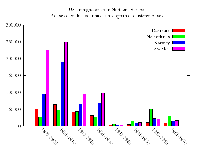
```
### 3
```ruby
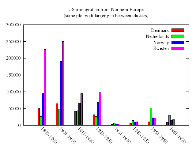
# set title "US immigration from Northern Europe\n(same plot with larger gap between clusters)"
# set style histogram gap 5
# replot
Numo.gnuplot do
set title:"US immigration from Northern Europe\n(same plot with larger gap between clusters)"
set :style, :histogram, gap:5
replot
end
```
### 4
```ruby
# # Stacked histograms
# #
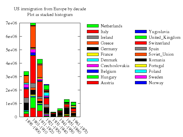
# set title "US immigration from Europe by decade\nPlot as stacked histogram"
# set key invert reverse Left outside
# set key autotitle columnheader
# set yrange [0:7e6]
# set auto x
# unset xtics
# set xtics nomirror rotate by -45 scale 0
# set style data histogram
# set style histogram rowstacked
# set style fill solid border -1
# set boxwidth 0.75
# #
# plot 'immigration.dat' using 2:xtic(1), for [i=3:22] '' using i
Numo.gnuplot do
set title:"US immigration from Europe by decade\nPlot as stacked histogram"
set :key, :invert, :reverse, :Left, :outside
set :key, autotitle:"columnheader"
set yrange:"[0:7e6]"
set auto:"x"
unset :xtics
set :xtics, :nomirror, rotate_by:-45, scale:0
set :style, :data, :histogram
set :style, histogram:"rowstacked"
set :style, :fill_solid, border:-1
set boxwidth:0.75
plot ["'immigration.dat'", using:'2:xtic(1)'],
"for [i=3:22] '' using i"
end
```
### 5
```ruby
# # Stacked histograms by percent
# #
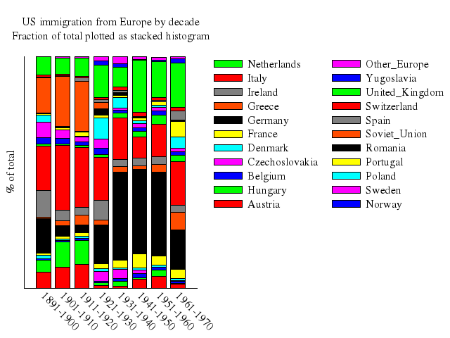
# set title "US immigration from Europe by decade\nFraction of total plotted as stacked histogram"
# set key invert reverse Left outside
# set yrange [0:100]
# set ylabel "% of total"
# unset ytics
# set grid y
# set border 3
# set style data histograms
# set style histogram rowstacked
# set style fill solid border -1
# set boxwidth 0.75
# #
# plot 'immigration.dat' using (100.*$2/$24):xtic(1) t column(2), \
# for [i=3:23] '' using (100.*column(i)/column(24)) title column(i)
Numo.gnuplot do
set title:"US immigration from Europe by decade\nFraction of total plotted as stacked histogram"
set :key, :invert, :reverse, :Left, :outside
set yrange:0..100
set ylabel:"% of total"
unset :ytics
set grid:"y"
set border:3
set :style, :data, :histograms
set :style, histogram:"rowstacked"
set :style, :fill_solid, border:-1
set boxwidth:0.75
plot ["'immigration.dat'", using:'(100.*$2/$24):xtic(1)', t_nq:'column(2)'],
"for [i=3:23] '' using (100.*column(i)/column(24)) title column(i)"
end
```
### 6
```ruby
# # Columnstacks
# # xtic labels should be picked up from column heads ('title column')
# # key titles should be picked up from row heads ('key(1)')
# #
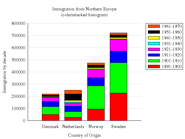
# set title "Immigration from Northern Europe\n(columstacked histogram)"
# set style histogram columnstacked
# set key noinvert box
# set yrange [0:*]
# set ylabel "Immigration by decade"
# set xlabel "Country of Origin"
# set tics scale 0.0
# set ytics
# unset xtics
# set xtics norotate nomirror
# plot 'immigration.dat' using 6 ti col, '' using 12 ti col, \
# '' using 13 ti col, '' using 14:key(1) ti col
Numo.gnuplot do
set title:"Immigration from Northern Europe\n(columstacked histogram)"
set :style, histogram:"columnstacked"
set :key, :noinvert, :box
set yrange:"[0:*]"
set ylabel:"Immigration by decade"
set xlabel:"Country of Origin"
set :tics, :scale, 0.0
set :ytics
unset :xtics
set :xtics, :norotate, :nomirror
plot ["'immigration.dat'", using:6, ti_nq:'col'],
["''", using:12, ti_nq:'col'],
["''", using:13, ti_nq:'col'],
["''", using:'14:key(1)', ti_nq:'col']
end
```
### 7
```ruby
# # 'newhistogram' keyword to plot
# #
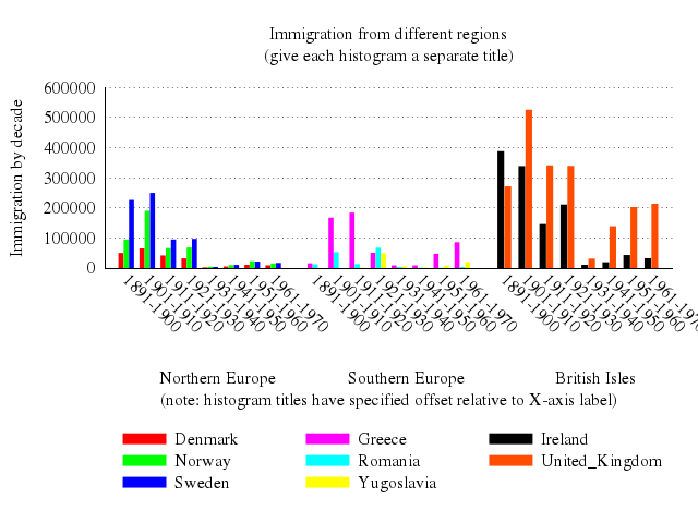
# set title "Immigration from different regions\n(give each histogram a separate title)"
# set key under nobox
# set style histogram clustered gap 1 title offset 2,0.25
# set style fill solid noborder
# set boxwidth 0.95
# unset xtics
# set xtics nomirror rotate by -45 scale 0
# set xlabel "(note: histogram titles have specified offset relative to X-axis label)" offset 0,-2
# set ytics
# set grid y
# set auto y
# plot \
# newhistogram "Northern Europe", \
# 'immigration.dat' using 6:xtic(1) t col, '' u 13 t col, '' u 14 t col, \
# newhistogram "Southern Europe", \
# '' u 9:xtic(1) t col, '' u 17 t col, '' u 22 t col, \
# newhistogram "British Isles", \
# '' u 10:xtic(1) t col, '' u 21 t col
Numo.gnuplot do
set title:"Immigration from different regions\n(give each histogram a separate title)"
set :key, "under", :nobox
set :style, :histogram, clustered_gap:1, title_offset:[2,0.25]
set :style, :fill_solid, :noborder
set boxwidth:0.95
unset :xtics
set :xtics, :nomirror, rotate_by:-45, scale:0
set xlabel:"(note: histogram titles have specified offset relative to X-axis label)", offset:[0,-2]
set :ytics
set grid:"y"
set auto:"y"
plot "newhistogram \"Northern Europe\"",
["'immigration.dat'", using:'6:xtic(1)', t_nq:'col'],
["''", u:13, t_nq:'col'],
["''", u:14, t_nq:'col'],
"newhistogram \"Southern Europe\"",
["''", u:'9:xtic(1)', t_nq:'col'],
["''", u:17, t_nq:'col'],
["''", u:22, t_nq:'col'],
"newhistogram \"British Isles\"",
["''", u:'10:xtic(1)', t_nq:'col'],
["''", u:21, t_nq:'col']
end
```
### 8
```ruby
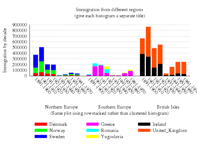
# set style histogram rows
# set boxwidth 0.8
# set yrange [0:900000]
# set xlabel "(Same plot using rowstacked rather than clustered histogram)"
# replot
Numo.gnuplot do
set :style, histogram:"rows"
set boxwidth:0.8
set yrange:0..900000
set xlabel:"(Same plot using rowstacked rather than clustered histogram)"
replot
end
```
## step functions
[Original Demo](http://gnuplot.sourceforge.net/demo_4.6/steps.html)
### 1
```ruby
# # This file will serve as the datafile used in demonstrating the
# # "plot with steps" option. Here is a gnuplot input file
# # which uses "plot with steps", inverse error function, normal
# # distribution function, and the inverse normal distribution
# # function.
#
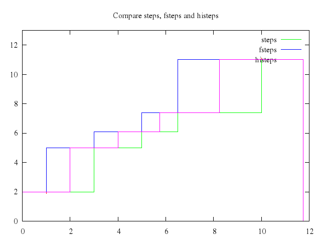
# set title "Compare steps, fsteps and histeps"
# plot [0:12][0:13] "steps.dat" notitle with points, \
# "steps.dat" title 'steps' with steps, \
# 'steps.dat' title 'fsteps' with fsteps, \
# 'steps.dat' title 'histeps' with histeps
Numo.gnuplot do
set title:"Compare steps, fsteps and histeps"
plot 0..12, 0..13,
["\"steps.dat\"", :notitle, with:"points"],
["\"steps.dat\"", title:'steps', with:"steps"],
["'steps.dat'", title:'fsteps', with:"fsteps"],
["'steps.dat'", title:'histeps', with:"histeps"]
end
```
### 2
```ruby
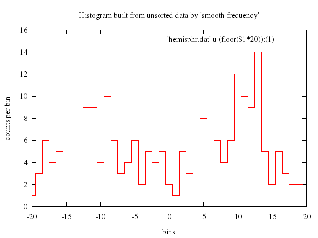
# set title "Histogram built from unsorted data by 'smooth frequency'"
# set ylabel 'counts per bin'
# set xlabel 'bins'
# plot 'hemisphr.dat' u (floor($1*20)):(1) smooth frequency with histeps
Numo.gnuplot do
set title:"Histogram built from unsorted data by 'smooth frequency'"
set ylabel:'counts per bin'
set xlabel:'bins'
plot "'hemisphr.dat'", u:'(floor($1*20)):(1)', smooth:"frequency", with:"histeps"
end
```
### 3
```ruby
# unset xlabel
# unset ylabel
#
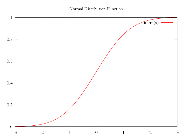
# set title "Normal Distribution Function"
# plot [-3:3][0:1] norm(x)
Numo.gnuplot do
unset :xlabel
unset :ylabel
set title:"Normal Distribution Function"
plot -3..3, 0..1,
"norm(x)"
end
```
### 4
```ruby
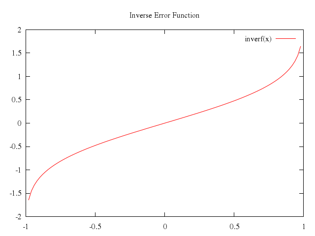
# set title "Inverse Error Function"
# plot [-1:1] inverf(x)
Numo.gnuplot do
set title:"Inverse Error Function"
plot -1..1,
"inverf(x)"
end
```
### 5
```ruby
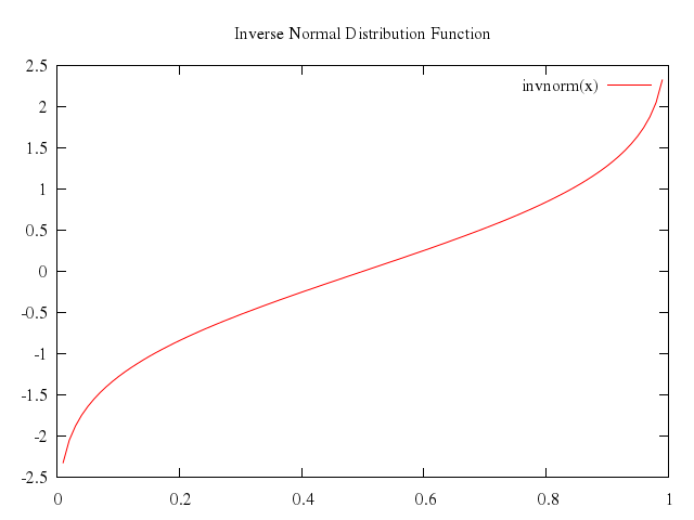
# set title "Inverse Normal Distribution Function"
# plot [0:1] invnorm(x)
Numo.gnuplot do
set title:"Inverse Normal Distribution Function"
plot 0..1,
"invnorm(x)"
end
```
## multiple axis scales
[Original Demo](http://gnuplot.sourceforge.net/demo_4.6/multiaxis.html)
### 1
```ruby
# # Use the 3rd plot of the electronics demo to show off
# # the use of multiple x and y axes in the same plot.
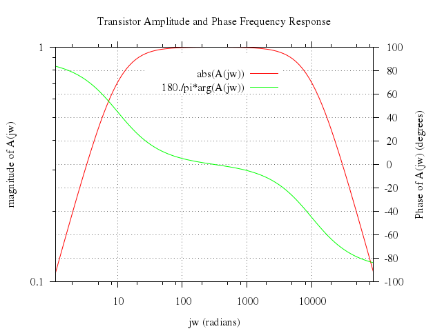
# #
# A(jw) = ({0,1}*jw/({0,1}*jw+p1)) * (1/(1+{0,1}*jw/p2))
# p1 = 10
# p2 = 10000
# set dummy jw
# set grid x y2
# set key center top title " "
# set logscale xy
# set log x2
# unset log y2
# set title "Transistor Amplitude and Phase Frequency Response"
# set xlabel "jw (radians)"
# set xrange [1.1 : 90000.0]
# set x2range [1.1 : 90000.0]
# set ylabel "magnitude of A(jw)"
# set y2label "Phase of A(jw) (degrees)"
# set ytics nomirror
# set y2tics
# set tics out
# set autoscale y
# set autoscale y2
# plot abs(A(jw)) axes x1y1, 180./pi*arg(A(jw)) axes x2y2
Numo.gnuplot do
run "A(jw) = ({0,1}*jw/({0,1}*jw+p1)) * (1/(1+{0,1}*jw/p2))"
run "p1 = 10"
run "p2 = 10000"
set dummy:"jw"
set :grid, "x y2"
set :key, :center, :top, title:" "
set logscale:"xy"
set log:"x2"
unset log:"y2"
set title:"Transistor Amplitude and Phase Frequency Response"
set xlabel:"jw (radians)"
set xrange:1.1..90000.0
set x2range:1.1..90000.0
set ylabel:"magnitude of A(jw)"
set y2label:"Phase of A(jw) (degrees)"
set :ytics, :nomirror
set :y2tics
set :tics, :out
set autoscale:"y"
set autoscale:"y2"
plot ["abs(A(jw))", axes:"x1y1"],
["180./pi*arg(A(jw))", axes:"x2y2"]
end
```
## mixing styles
[Original Demo](http://gnuplot.sourceforge.net/demo_4.6/using.html)
### 1
```ruby
# # Requires data file "using.dat" from this directory,
# # so change current working directory to this directory before running.
# #
#
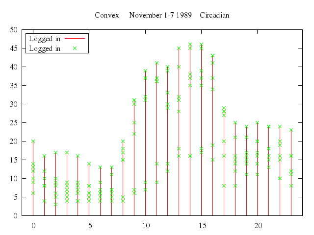
# set title "Convex November 1-7 1989 Circadian"
# set key left box
# set xrange[-1:24]
# plot 'using.dat' using 2:4 title "Logged in" with impulses,\
# 'using.dat' using 2:4 title "Logged in" with points
Numo.gnuplot do
set title:"Convex November 1-7 1989 Circadian"
set :key, :left, :box
set xrange:-1..24
plot ["'using.dat'", using:[2,4], title:"Logged in", with:"impulses"],
["'using.dat'", using:[2,4], title:"Logged in", with:"points"]
end
```
### 2
```ruby
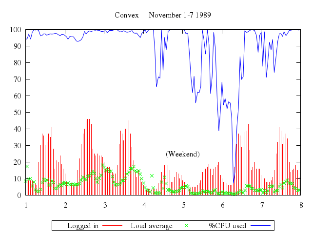
# set xrange [1:8]
# #set xdtic
# set title "Convex November 1-7 1989"
# set key below
# set label "(Weekend)" at 5,25 center
# plot 'using.dat' using 3:4 title "Logged in" with impulses,\
# 'using.dat' using 3:5 t "Load average" with points,\
# 'using.dat' using 3:6 t "%CPU used" with lines
Numo.gnuplot do
set xrange:1..8
set title:"Convex November 1-7 1989"
set :key, "below"
set label:"(Weekend)", at:[5,25], center:true
plot ["'using.dat'", using:[3,4], title:"Logged in", with:"impulses"],
["'using.dat'", using:[3,5], t:"Load average", with:"points"],
["'using.dat'", using:[3,6], t:"%CPU used", with:"lines"]
end
```
## variable size points
[Original Demo](http://gnuplot.sourceforge.net/demo_4.6/pointsize.html)
### 1
```ruby
# # Read individual point sizes from extra column of input file
# # Ethan A Merritt - October 2004
# #
# unset key
# unset border
# unset yzeroaxis
# unset xtics
# unset ytics
# unset ztics
#
# #
# # plot a 2D map with locations marked by variable sized points
# #
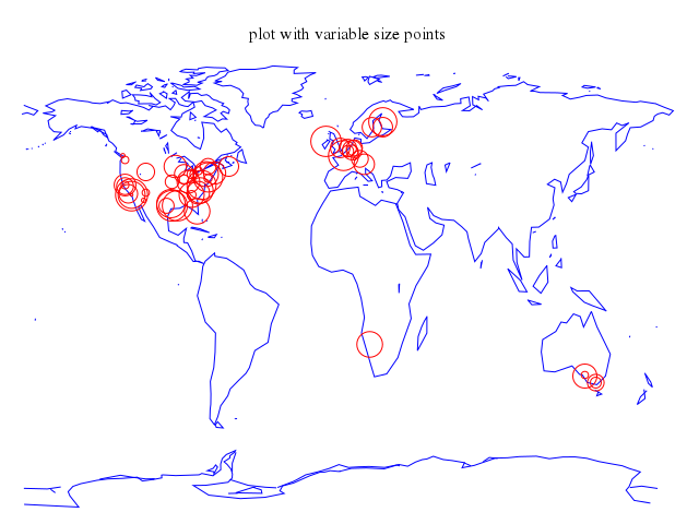
# set title "plot with variable size points"
# plot 'world.dat' with lines lt 3, \
# 'world.cor' using 1:2:(5.*rand(0)) with points lt 1 pt 6 ps variable
Numo.gnuplot do
unset :key
unset :border
unset :yzeroaxis
unset :xtics
unset :ytics
unset :ztics
set title:"plot with variable size points"
plot ["'world.dat'", with:"lines", lt:3],
["'world.cor'", using:'1:2:(5.*rand(0))', with:"points", lt:1, pt:6, ps:"variable"]
end
```
### 2
```ruby
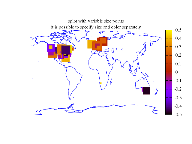
# set title "splot with variable size points\nit is possible to specify size and color separately"
# set view map
# unset hidden3d
# splot 'world.dat' using 1:2:(0) with lines lt 3, \
# 'world.cor' using 1:2:(0.5-rand(0)):(5.*rand(0)) with points pt 5 ps var lt palette
Numo.gnuplot do
set title:"splot with variable size points\nit is possible to specify size and color separately"
set view:'map'
unset :hidden3d
splot ["'world.dat'", using:'1:2:(0)', with:"lines", lt:3],
["'world.cor'", using:'1:2:(0.5-rand(0)):(5.*rand(0))', with:"points", pt:5, ps:"var", lt:true, palette:true]
end
```
### 3
```ruby
# # plot a '3D version using spherical coordinate system' of the world.
# set angles degrees
# set title "3D version using spherical coordinate system"
# set ticslevel 0
# set view 70,40,0.8,1.2
# set mapping spherical
# set parametric
# set samples 32
# set isosamples 9
# set urange [-90:90]
# set vrange [0:360]
# splot cos(u)*cos(v),cos(u)*sin(v),sin(u) with lines lt 5,\
# 'world.dat' with lines lt 3, \
# 'world.cor' using 1:2:(1):(5.*rand(0)) with points lt 1 pt 6 ps variable
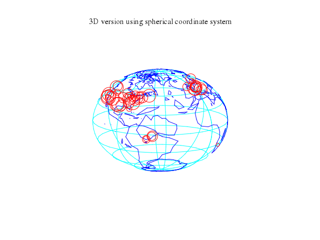
Numo.gnuplot do
set angles:"degrees"
set title:"3D version using spherical coordinate system"
set ticslevel:0
set view:[70,40,0.8,1.2]
set mapping:"spherical"
set :parametric
set samples:32
set isosamples:9
set urange:-90..90
set vrange:0..360
splot "cos(u)*cos(v)",
"cos(u)*sin(v)",
["sin(u)", with:"lines", lt:5],
["'world.dat'", with:"lines", lt:3],
["'world.cor'", using:'1:2:(1):(5.*rand(0))', with:"points", lt:1, pt:6, ps:"variable"]
end
```
### 4
```ruby
# # hidden3d still not working fully
# # pointsize is now handled, but axes are never obscured
# #
# set title "3D solid version through hiddenlining"
# set hidden3d
# set arrow from 0,0,-1.2 to 0,0,1.2 lt 5 lw 2
# set arrow from -1.2, 0, 0 to 1.2, 0, 0 nohead lt 5 lw 1
# set arrow from 0, -1.2, 0 to 0, 1.2, 0 nohead lt 5 lw 1
# splot cos(u)*cos(v),-cos(u)*sin(v),sin(u) with lines lt 5,\
# 'world.dat' u 1:2:(1.001) with lines lt 3, \
# 'world.cor' using 1:2:(1):(5.*rand(0)) with points lt 1 pt 6 ps var
Numo.gnuplot do
set title:"3D solid version through hiddenlining"
set :hidden3d
set :arrow, from:[0,0,-1.2], to:[0,0,1.2], lt:5, lw:2
set :arrow, from:[-1.2,0,0], to:[1.2,0,0], nohead:true, lt:5, lw:1
set :arrow, from:[0,-1.2,0], to:[0,1.2,0], nohead:true, lt:5, lw:1
splot "cos(u)*cos(v)",
"-cos(u)*sin(v)",
["sin(u)", with:"lines", lt:5],
["'world.dat'", u:'1:2:(1.001)', with:"lines", lt:3],
["'world.cor'", using:'1:2:(1):(5.*rand(0))', with:"points", lt:1, pt:6, ps:"var"]
end
```

## parametric functions
[Original Demo](http://gnuplot.sourceforge.net/demo_4.6/param.html)
### 1
```ruby
# # Show some of the new parametric capabilities.
# #
# set parametric
# set dummy t
# set autoscale
# set samples 160
# set title ""
# set key box
# set key below
# plot t,sin(t)/t title "t,sin(t)/t or sin(x)/x"
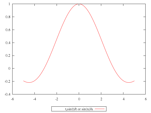
Numo.gnuplot do
set :parametric
set dummy:"t"
set :autoscale
set samples:160
set title:""
set :key, :box
set :key, "below"
plot "t",
["sin(t)/t", title:"t,sin(t)/t or sin(x)/x"]
end
```
### 2
```ruby
# plot sin(t)/t,t
Numo.gnuplot do
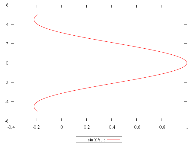
plot "sin(t)/t",
"t"
end
```
### 3
```ruby
# plot sin(t),cos(t)
Numo.gnuplot do
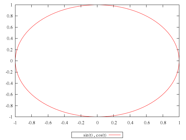
plot "sin(t)",
"cos(t)"
end
```
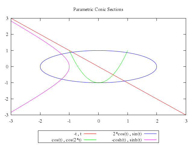
### 4
```ruby
# set xrange [-3:3]
# set yrange [-3:3]
# set title "Parametric Conic Sections"
# plot -t,t,cos(t),cos(2*t),2*cos(t),sin(t),-cosh(t),sinh(t)
Numo.gnuplot do
set xrange:-3..3
set yrange:-3..3
set title:"Parametric Conic Sections"
plot "-t",
"t",
"cos(t)",
"cos(2*t)",
"2*cos(t)",
"sin(t)",
"-cosh(t)",
"sinh(t)"
end
```
### 5
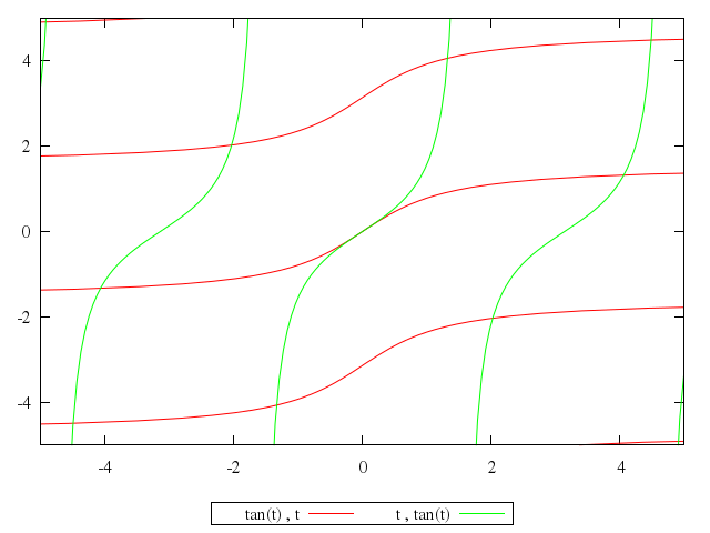
```ruby
# set title ""
#
# set xrange [-5:5]
# set yrange [-5:5]
# plot tan(t),t,t,tan(t)
Numo.gnuplot do
set title:""
set xrange:-5..5
set yrange:-5..5
plot "tan(t)",
"t",
"t",
"tan(t)"
end
```
### 6
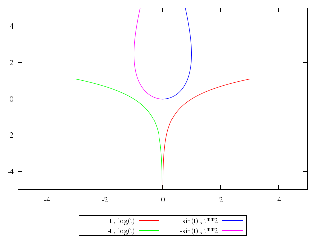
```ruby
# set trange [0.00001:3]
# plot t,log(t),-t,log(t),sin(t),t**2,-sin(t),t**2
Numo.gnuplot do
set trange:0.00001..3
plot "t",
"log(t)",
"-t",
"log(t)",
"sin(t)",
"t**2",
"-sin(t)",
"t**2"
end
```
### 7
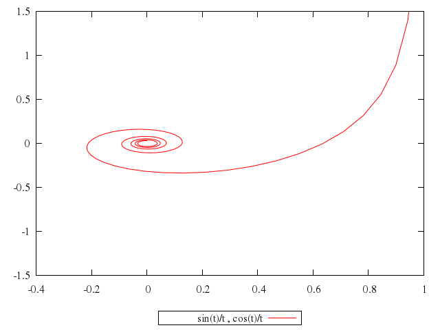
```ruby
# set autoscale x
# set yrange [-1.5:1.5]
# set trange [0.0001:10*pi]
# plot sin(t)/t,cos(t)/t
Numo.gnuplot do
set autoscale:"x"
set yrange:-1.5..1.5
set trange:"[0.0001:10*pi]"
plot "sin(t)/t",
"cos(t)/t"
end
```
## vector fields
[Original Demo](http://gnuplot.sourceforge.net/demo_4.6/vector.html)
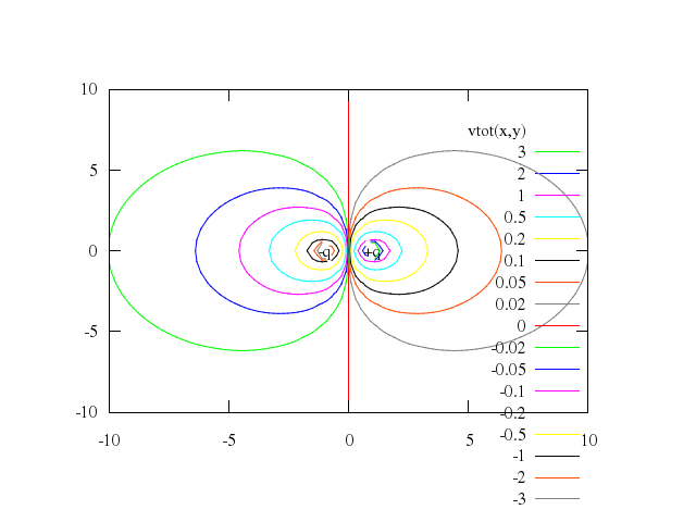
### 1
```ruby
# # This file demonstrates
# # -1- saving contour lines as a gnuplottable file
# # -2- plotting a vector field on the same graph
# # -3- manipulating columns using the '$1,$2' syntax.
# # the example is taken here from Physics is the display of equipotential
# # lines and electrostatic field for a dipole (+q,-q)
#
# print "\n This file demonstrates"
# print " -1- saving contour lines as a gnuplottable file"
# print " -2- plotting a vector field on the same graph"
# print " -3- manipulating columns using the '$1,$2' syntax."
# print " the example is taken here from Physics is the display of equipotential"
# print " lines and electrostatic field for a dipole (+q,-q)"
# #
# r(x,y)=sqrt(x*x+y*y)
# v1(x,y)= q1/(r((x-x0),y))
# v2(x,y)= q2/(r((x+x0),y))
# #
# vtot(x,y)=v1(x,y)+v2(x,y)
# #
# e1x(x,y)= q1*(x-x0)/r(x-x0,y)**3
# e1y(x,y)= q1*(y)/r(x-x0,y)**3
# e2x(x,y)= q2*(x+x0)/r(x+x0,y)**3
# e2y(x,y)= q2*(y)/r(x+x0,y)**3
# etotx(x,y)=e1x(x,y)+e2x(x,y)
# etoty(x,y)=e1y(x,y)+e2y(x,y)
# enorm(x,y)=sqrt(etotx(x,y)*etotx(x,y)+etoty(x,y)*etoty(x,y))
# dx1(x,y)=coef*etotx(x,y)/enorm(x,y)
# dy1(x,y)=coef*etoty(x,y)/enorm(x,y)
# dx2(x,y)=coef*etotx(x,y)
# dy2(x,y)=coef*etoty(x,y)
# #
# coef=.7
# x0=1.
# q1=1
# q2=-1
# xmin=-10.
# xmax=10.
# ymin=-10.
# ymax=10.
# #
# reset
# unset autoscale
# set xr [xmin:xmax]
# set yr [ymin:ymax]
# set isosam 31,31
# #set view 0, 0, 1, 1
# set view map
# unset surface
# set contour base
# set cntrparam order 4
# set cntrparam linear
# set cntrparam levels discrete -3,-2 ,-1 ,-0.5 ,-0.2 ,-0.1 ,-0.05 ,-0.02 ,0 ,0.02 ,0.05 ,0.1 ,0.2 ,0.5 ,1 ,2 ,3
# set cntrparam points 5
# #
# set label "-q" at -1,0 center
# set label "+q" at 1,0 center
# splot vtot(x,y) w l
Numo.gnuplot do
run "r(x,y)=sqrt(x*x+y*y)"
run "v1(x,y)= q1/(r((x-x0),y))"
run "v2(x,y)= q2/(r((x+x0),y))"
run "vtot(x,y)=v1(x,y)+v2(x,y)"
run "e1x(x,y)= q1*(x-x0)/r(x-x0,y)**3"
run "e1y(x,y)= q1*(y)/r(x-x0,y)**3"
run "e2x(x,y)= q2*(x+x0)/r(x+x0,y)**3"
run "e2y(x,y)= q2*(y)/r(x+x0,y)**3"
run "etotx(x,y)=e1x(x,y)+e2x(x,y)"
run "etoty(x,y)=e1y(x,y)+e2y(x,y)"
run "enorm(x,y)=sqrt(etotx(x,y)*etotx(x,y)+etoty(x,y)*etoty(x,y))"
run "dx1(x,y)=coef*etotx(x,y)/enorm(x,y)"
run "dy1(x,y)=coef*etoty(x,y)/enorm(x,y)"
run "dx2(x,y)=coef*etotx(x,y)"
run "dy2(x,y)=coef*etoty(x,y)"
run "coef=.7"
run "x0=1."
run "q1=1"
run "q2=-1"
run "xmin=-10."
run "xmax=10."
run "ymin=-10."
run "ymax=10."
reset
unset :autoscale
set xr:"[xmin:xmax]"
set yr:"[ymin:ymax]"
set isosam:[31,31]
set view:'map'
unset :surface
set contour:"base"
set :cntrparam, order:4
set :cntrparam, "linear"
set :cntrparam, :levels, discrete:[-3,-2,-1,-0.5,-0.2,-0.1,-0.05,-0.02,0,0.02,0.05,0.1,0.2,0.5,1,2,3]
set :cntrparam, points:5
set label:"-q", at:[-1,0], center:true
set label:"+q", at:[1,0], center:true
splot "vtot(x,y)", w:"l"
end
```
### 2
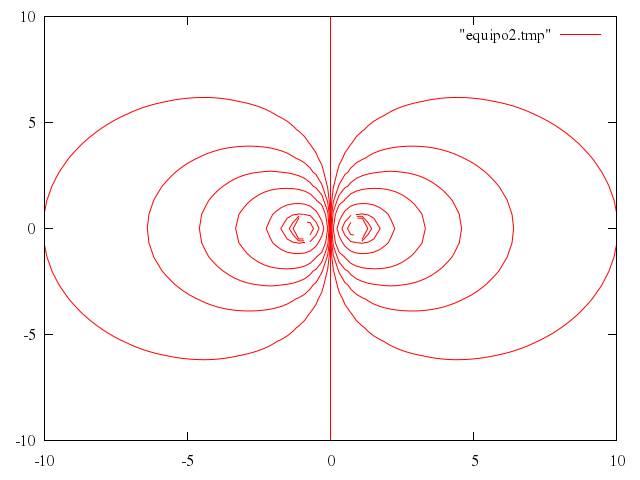
```ruby
# print "Now create a file with equipotential lines"
#
# set table "equipo2.tmp"
# replot
# unset table
# reset
#
# plot "equipo2.tmp" w l
Numo.gnuplot do
set table:"equipo2.tmp"
replot
unset :table
reset
plot "\"equipo2.tmp\"", w:"l"
end
```
### 3
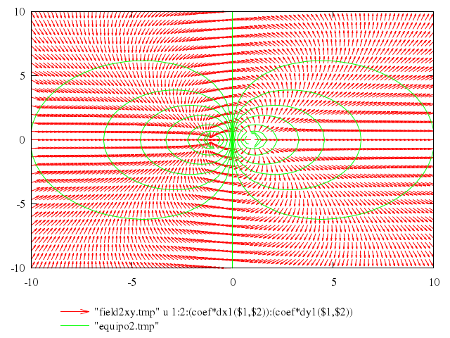
```ruby
# print "Now create a x/y datafile for plotting with vectors "
# print "and display vectors parallel to the electrostatic field"
# set isosam 31,31
#
# set table "field2xy.tmp"
# splot vtot(x,y) w l
# unset table
#
# unset autoscale
# set xr [xmin:xmax]
# set yr [ymin:ymax]
# set isosam 31,31
# set key under Left reverse
# plot "field2xy.tmp" u 1:2:(coef*dx1($1,$2)):(coef*dy1($1,$2)) w vec, \
# "equipo2.tmp" w l
Numo.gnuplot do
set isosam:[31,31]
set table:"field2xy.tmp"
splot "vtot(x,y)", w:"l"
unset :table
unset :autoscale
set xr:"[xmin:xmax]"
set yr:"[ymin:ymax]"
set isosam:[31,31]
set :key, "under", :Left, :reverse
plot ["\"field2xy.tmp\"", u:'1:2:(coef*dx1($1,$2)):(coef*dy1($1,$2))', w:"vec"],
["\"equipo2.tmp\"", w:"l"]
end
```
## circles
[Original Demo](http://gnuplot.sourceforge.net/demo_4.6/circles.html)
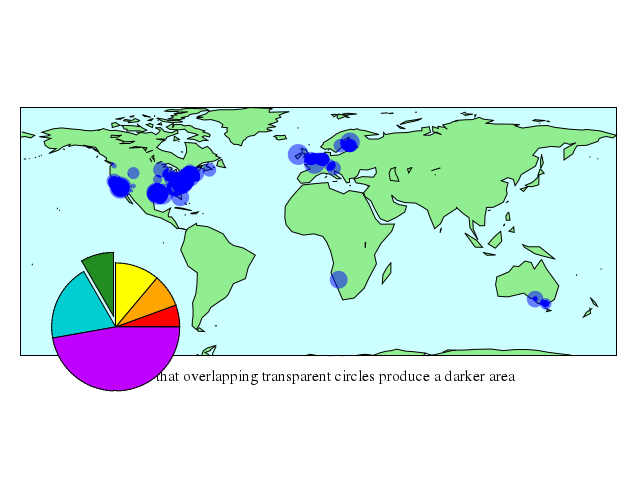
### 1
```ruby
# # demo for the use of "set object circle" and "plot ... with circles"
# #
# # Ethan A Merritt, Ralf Juengling - 2007,2008
#
# if ((GPVAL_VERSION == 4.3 || GPVAL_VERSION == 4.2) \
# && (!strstrt(GPVAL_COMPILE_OPTIONS,"+OBJECTS"))) \
# print ">>> Skipping demo <<<\n" ; \
# print "This copy of gnuplot was built without support for circles\n" ; \
# exit ;
#
# set size ratio -1
# set style fill solid 1.0 border -1
#
# set obj 10 circle arc [ 0 : 20] fc rgb "red"
# set obj 11 circle arc [ 20 : 50] fc rgb "orange"
# set obj 12 circle arc [ 50 : 90] fc rgb "yellow"
# set obj 13 circle arc [ 90 : 120] fc rgb "forest-green"
# set obj 14 circle arc [120 : 190] fc rgb "dark-turquoise"
# set obj 15 circle arc [190 : 360] fc rgb "dark-magenta"
#
# set obj 10 circle at screen .18,.32 size screen .10 front
# set obj 11 circle at screen .18,.32 size screen .10 front
# set obj 12 circle at screen .18,.32 size screen .10 front
# set obj 13 circle at screen .1767,.342 size screen .10 front
# set obj 14 circle at screen .18,.32 size screen .10 front
# set obj 15 circle at screen .18,.32 size screen .10 front
#
# set obj 20 rect from graph 0,0 to graph 1,1 behind fc rgb "cyan" fs solid 0.2
#
# # plot world map and correspondent locations as a circle
# set title ""
# set xlabel "Note that overlapping transparent circles produce a darker area"
# unset key
# unset xtics
# unset ytics
# set border
#
# set yrange [-70:*]
#
# plot 'world.dat' with filledcurves lc rgb "light-green" , \
# 'world.cor' using 1:2:(7.*rand(0)) with circles lt 3 \
# fs transparent solid 0.5 noborder
Numo.gnuplot do
set :size, :ratio, -1
set :style, fill_solid:1.0, border:-1
set :obj, 10, :circle, arc:0..20, fc_rgb:"red"
set :obj, 11, :circle, arc:20..50, fc_rgb:"orange"
set :obj, 12, :circle, arc:50..90, fc_rgb:"yellow"
set :obj, 13, :circle, arc:90..120, fc_rgb:"forest-green"
set :obj, 14, :circle, arc:120..190, fc_rgb:"dark-turquoise"
set :obj, 15, :circle, arc:190..360, fc_rgb:"dark-magenta"
set :obj, 10, :circle, at_screen:[0.18,0.32], size_screen:0.10, front:true
set :obj, 11, :circle, at_screen:[0.18,0.32], size_screen:0.10, front:true
set :obj, 12, :circle, at_screen:[0.18,0.32], size_screen:0.10, front:true
set :obj, 13, :circle, at_screen:[0.1767,0.342], size_screen:0.10, front:true
set :obj, 14, :circle, at_screen:[0.18,0.32], size_screen:0.10, front:true
set :obj, 15, :circle, at_screen:[0.18,0.32], size_screen:0.10, front:true
set :obj, 20, "rect", from_graph:[0,0], to_graph:[1,1], behind:true, fc_rgb:"cyan", fs_solid:0.2
set title:""
set xlabel:"Note that overlapping transparent circles produce a darker area"
unset :key
unset :xtics
unset :ytics
set :border
set yrange:"[-70:*]"
plot ["'world.dat'", with:"filledcurves", lc_rgb:"light-green"],
["'world.cor'", using:'1:2:(7.*rand(0))', with:"circles", lt:3, fs:"transparent", solid:0.5, noborder:true]
end
```
### 2
```ruby
# # by Peter Juhasz - 2010
#
# reset
#
# set style fill solid 1.0 border -1
# set size ratio -1
#
# # Plot pie charts on top of the map of the world.
# # The pie segments are read from a data file.
# # Each segment has to be specified with a start and end angle.
#
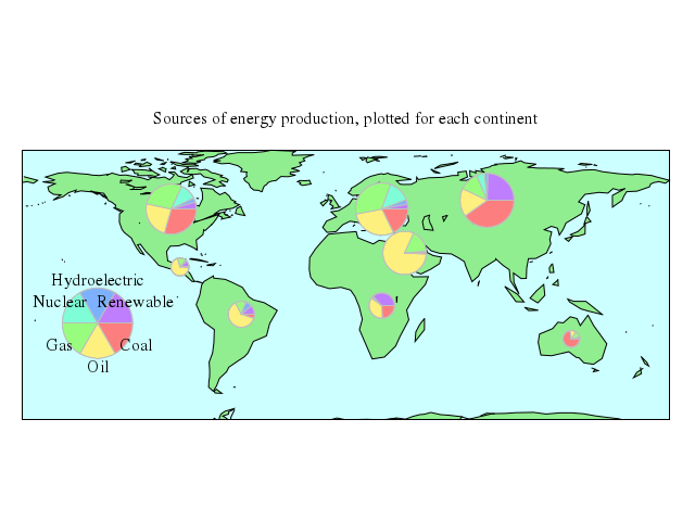
# set title "Sources of energy production, plotted for each continent"
#
# unset key
# unset xtics
# unset ytics
# set border
#
# set yrange [-70:*]
# set palette model HSV func gray*0.75, 0.5, 0.99
# unset colorbox
# r = 0.01
# types = 6
# keyx = -137.
# keyy = -15.
# keyr = 25.
#
# set obj 20 rect from graph 0,0 to graph 1,1 behind fc rgb "cyan" fs solid 0.2
# set angle degree
#
# plot 'world.dat' with filledcurves lc rgb "light-green" notit, \
# 'energy_circles.dat' using 2:1:(sqrt($9)*r):6:($6+$7):5 \
# with circles lc pal fs solid 1.0 border rgb "gray",\
# for [i=0:types-1] '' using (keyx):(keyy):(keyr-5):(-(i+1)*360./types):(-(i)*360./types):5 \
# every ::i::i with circles lc pal fs solid 1.0 border rgb "gray",\
# for [i=0:types-1] '' using \
# (keyx+keyr*cos(-(i+0.5)*360./types)):(keyy+keyr*sin(-(i+0.5)*360./types)):4 \
# every ::i::i with labels
Numo.gnuplot do
reset
set :style, fill_solid:1.0, border:-1
set :size, :ratio, -1
set title:"Sources of energy production, plotted for each continent"
unset :key
unset :xtics
unset :ytics
set :border
set yrange:"[-70:*]"
set :palette, model:"HSV", func:'gray*0.75,0.5,0.99'
unset :colorbox
run "r = 0.01"
run "types = 6"
run "keyx = -137."
run "keyy = -15."
run "keyr = 25."
set :obj, 20, "rect", from_graph:[0,0], to_graph:[1,1], behind:true, fc_rgb:"cyan", fs_solid:0.2
set angle:"degree"
plot ["'world.dat'", with:"filledcurves", lc_rgb:"light-green", notit:true],
["'energy_circles.dat'", using:'2:1:(sqrt($9)*r):6:($6+$7):5', with:"circles", lc:true, pal:true, fs_solid:1.0, border_rgb:"gray"],
"for [i=0:types-1] '' using (keyx):(keyy):(keyr-5):(-(i+1)*360./types):(-(i)*360./types):5 every ::i::i with circles lc pal fs solid 1.0 border rgb \"gray\"",
"for [i=0:types-1] '' using (keyx+keyr*cos(-(i+0.5)*360./types)):(keyy+keyr*sin(-(i+0.5)*360./types)):4 every ::i::i with labels"
end
```
### 3
```ruby
# # by Ralf Juengling - 2008
#
# reset
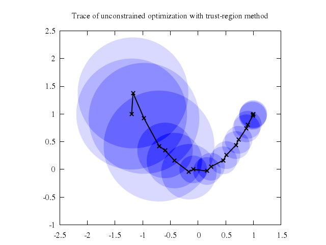
# set title "Trace of unconstrained optimization with trust-region method"
# unset key
# set size ratio -1
# set xrange [-2.5:1.5]
# set yrange [-1:2.5]
# plot 'optimize.dat' with circles lc rgb "blue" fs transparent solid 0.15 noborder,\
# 'optimize.dat' u 1:2 with linespoints lw 2 lc rgb "black"
Numo.gnuplot do
reset
set title:"Trace of unconstrained optimization with trust-region method"
unset :key
set :size, :ratio, -1
set xrange:-2.5..1.5
set yrange:-1..2.5
plot ["'optimize.dat'", with:"circles", lc_rgb:"blue", fs:"transparent", solid:0.15, noborder:true],
["'optimize.dat'", u:[1,2], with:"linespoints", lw:2, lc_rgb:"black"]
end
```
### 4
```ruby
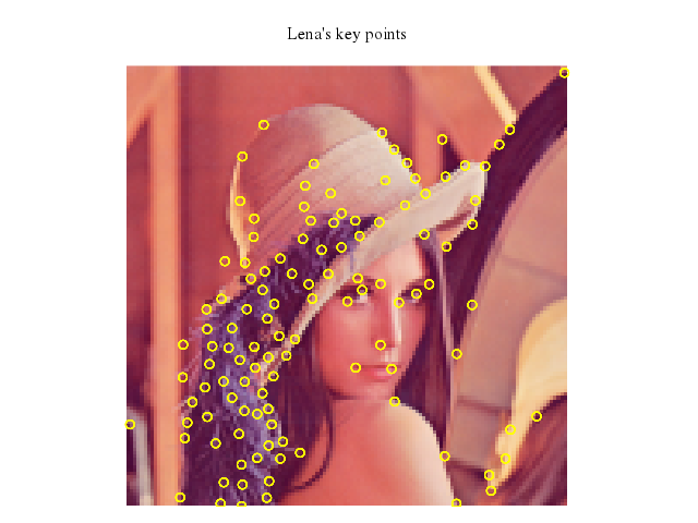
# reset
# set size ratio -1
# set title "Lena's key points"
# unset xtics
# unset ytics
# unset key
# unset border
# set yrange [] reverse
#
# plot 'lena.rgb' binary array=(128,128) dx=4 dy=4 format='%uchar' with rgbimage, \
# 'lena-keypoints.bin' binary format='%double' with circles lc rgb "yellow"
Numo.gnuplot do
reset
set :size, :ratio, -1
set title:"Lena's key points"
unset :xtics
unset :ytics
unset :key
unset :border
set yrange:"[]", reverse:true
plot ["'lena.rgb'", binary:'array=(128,128) dx=4 dy=4 format="%uchar"', with:"rgbimage"],
["'lena-keypoints.bin'", binary:'format="%double"', with:"circles", lc_rgb:"yellow"]
end
```
### 5
```ruby
# reset
# set size ratio -1
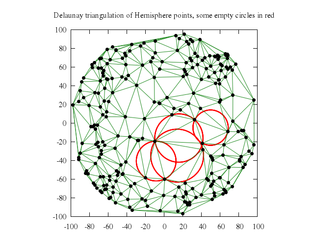
# set title "Delaunay triangulation of Hemisphere points, some empty circles in red"
# unset key
#
# plot 'empty-circles.dat' with circles lw 2 lc rgb "red", \
# 'delaunay-edges.dat' with lines lc rgb "forest-green", \
# 'hemisphr.dat' u (100*$1):(100*$2) with points pt 7 lc rgb "black"
Numo.gnuplot do
reset
set :size, :ratio, -1
set title:"Delaunay triangulation of Hemisphere points, some empty circles in red"
unset :key
plot ["'empty-circles.dat'", with:"circles", lw:2, lc_rgb:"red"],
["'delaunay-edges.dat'", with:"lines", lc_rgb:"forest-green"],
["'hemisphr.dat'", u:'(100*$1):(100*$2)', with:"points", pt:7, lc_rgb:"black"]
end
```
## approximation
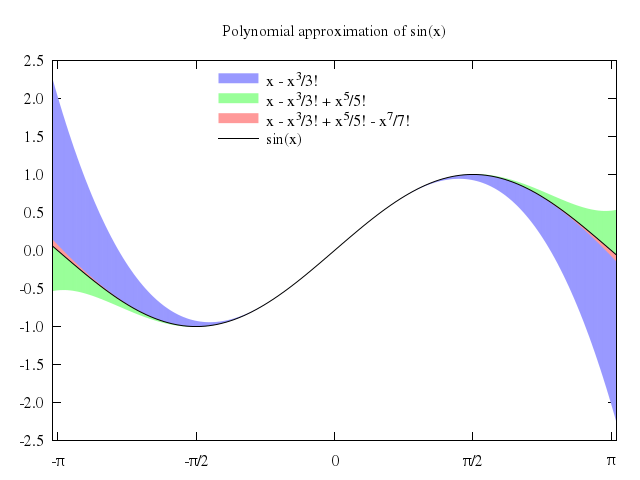
[Original Demo](http://gnuplot.sourceforge.net/demo_4.6/approximate.html)
### 1
```ruby
# # Show use of pseudodata mechanism '+' to use plot styles with more than
# # one relevant value per x coordinate. In this example we use the style
# # "filledcurves" to show the difference between two analytic functions.
# # This corresponds to the specification of multiple columns in the
# # 'using' option for input from data files.
# #
# #
# approx_1(x) = x - x**3/6
# approx_2(x) = x - x**3/6 + x**5/120
# approx_3(x) = x - x**3/6 + x**5/120 - x**7/5040
#
# label1 = "x - {x^3}/3!"
# label2 = "x - {x^3}/3! + {x^5}/5!"
# label3 = "x - {x^3}/3! + {x^5}/5! - {x^7}/7!"
#
# #
# set termoption enhanced
# set encoding utf8
# #
# set title "Polynomial approximation of sin(x)"
# set key Left center top reverse
# set xrange [ -3.2 : 3.2 ]
# set xtics ("-π" -pi, "-π/2" -pi/2, 0, "π/2" pi/2, "π" pi)
# set format y "%.1f"
# set samples 500
# set style fill solid 0.4 noborder
#
# plot '+' using 1:(sin($1)):(approx_1($1)) with filledcurve title label1 lt 3, \
# '+' using 1:(sin($1)):(approx_2($1)) with filledcurve title label2 lt 2, \
# '+' using 1:(sin($1)):(approx_3($1)) with filledcurve title label3 lt 1, \
# sin(x) with lines lw 1 lc rgb "black"
Numo.gnuplot do
run "approx_1(x) = x - x**3/6"
run "approx_2(x) = x - x**3/6 + x**5/120"
run "approx_3(x) = x - x**3/6 + x**5/120 - x**7/5040"
run "label1 = \"x - {x^3}/3!\""
run "label2 = \"x - {x^3}/3! + {x^5}/5!\""
run "label3 = \"x - {x^3}/3! + {x^5}/5! - {x^7}/7!\""
set :termoption, :enhanced
set encoding:"utf8"
set title:"Polynomial approximation of sin(x)"
set :key, :Left, :center, :top, :reverse
set xrange:-3.2..3.2
set xtics:'("-π" -pi, "-π/2" -pi/2, 0, "π/2" pi/2, "π" pi)'
set format_y:"%.1f"
set samples:500
set :style, fill_solid:0.4, noborder:true
plot ["'+'", using:'1:(sin($1)):(approx_1($1))', with:"filledcurve", title_nq:'label1', lt:3],
["'+'", using:'1:(sin($1)):(approx_2($1))', with:"filledcurve", title_nq:'label2', lt:2],
["'+'", using:'1:(sin($1)):(approx_3($1))', with:"filledcurve", title_nq:'label3', lt:1],
["sin(x)", with:"lines", lw:1, lc_rgb:"black"]
end
```
## B-splines
[Original Demo](http://gnuplot.sourceforge.net/demo_4.6/spline.html)
### 1
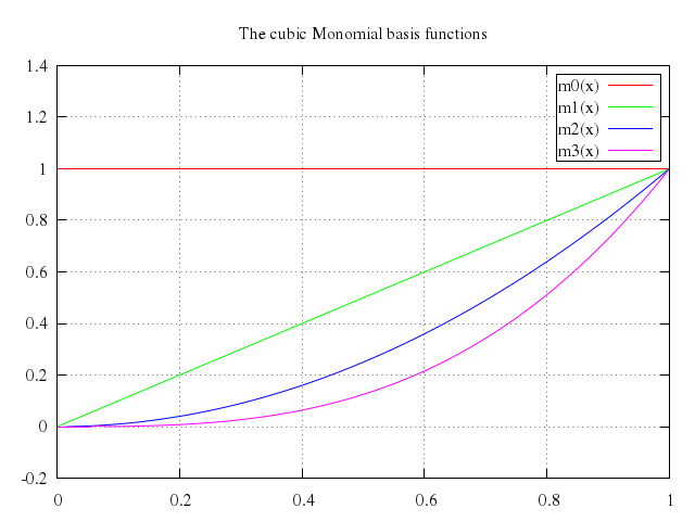
```ruby
# # Some curve plotting using common cubic polynomial basis function for cagd.
# #
# # Gershon Elber, Aug. 1992
# #
# set xrang [0:1]
# set grid
# set key box
#
# set yrange[-0.2:1.4]
# m0(x) = 1
# m1(x) = x
# m2(x) = x**2
# m3(x) = x**3
# set title "The cubic Monomial basis functions"
# plot m0(x), m1(x), m2(x), m3(x)
Numo.gnuplot do
set xrang:0..1
set :grid
set :key, :box
set yrange:-0.2..1.4
run "m0(x) = 1"
run "m1(x) = x"
run "m2(x) = x**2"
run "m3(x) = x**3"
set title:"The cubic Monomial basis functions"
plot "m0(x)",
"m1(x)",
"m2(x)",
"m3(x)"
end
```
### 2
```ruby
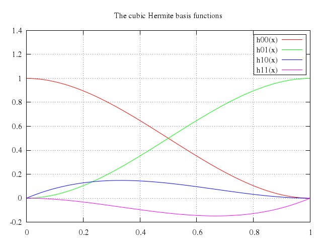
# h00(x) = x**2 * ( 2 * x - 3) + 1
# h01(x) = -x**2 * (2 * x - 3)
# h10(x) = x * (x - 1)**2
# h11(x) = x**2 * (x - 1)
#
# set title "The cubic Hermite basis functions"
# plot h00(x), h01(x), h10(x), h11(x)
Numo.gnuplot do
run "h00(x) = x**2 * ( 2 * x - 3) + 1"
run "h01(x) = -x**2 * (2 * x - 3)"
run "h10(x) = x * (x - 1)**2"
run "h11(x) = x**2 * (x - 1)"
set title:"The cubic Hermite basis functions"
plot "h00(x)",
"h01(x)",
"h10(x)",
"h11(x)"
end
```
### 3
```ruby
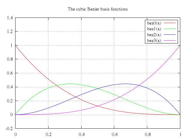
# bez0(x) = (1 - x)**3
# bez1(x) = 3 * (1 - x)**2 * x
# bez2(x) = 3 * (1 - x) * x**2
# bez3(x) = x**3
# set title "The cubic Bezier basis functions"
# plot bez0(x), bez1(x), bez2(x), bez3(x)
Numo.gnuplot do
run "bez0(x) = (1 - x)**3"
run "bez1(x) = 3 * (1 - x)**2 * x"
run "bez2(x) = 3 * (1 - x) * x**2"
run "bez3(x) = x**3"
set title:"The cubic Bezier basis functions"
plot "bez0(x)",
"bez1(x)",
"bez2(x)",
"bez3(x)"
end
```
### 4
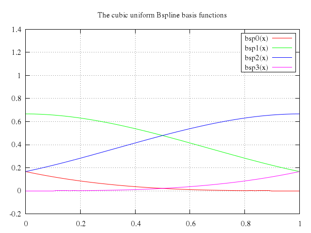
```ruby
# bsp0(x) = ( 1 - 3 * x + 3 * x**2 - x**3 ) / 6;
# bsp1(x) = ( 4 - 6 * x**2 + 3 * x**3 ) / 6;
# bsp2(x) = ( 1 + 3 * x + 3 * x**2 - 3 * x**3 ) / 6
# bsp3(x) = x**3 / 6
# set title "The cubic uniform Bspline basis functions"
# plot bsp0(x), bsp1(x), bsp2(x), bsp3(x)
Numo.gnuplot do
run "bsp0(x) = ( 1 - 3 * x + 3 * x**2 - x**3 ) / 6;"
run "bsp1(x) = ( 4 - 6 * x**2 + 3 * x**3 ) / 6;"
run "bsp2(x) = ( 1 + 3 * x + 3 * x**2 - 3 * x**3 ) / 6"
run "bsp3(x) = x**3 / 6"
set title:"The cubic uniform Bspline basis functions"
plot "bsp0(x)",
"bsp1(x)",
"bsp2(x)",
"bsp3(x)"
end
```
### 5
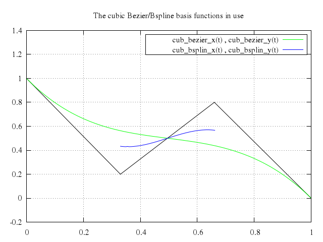
```ruby
# y0 = 1
# y1 = 0.2
# y2 = 0.8
# y3 = 0
#
# x0 = 0
# x1 = 0.33
# x2 = 0.66
# x3 = 1
#
# xv0 = -0.3
# yv0 = 0.5
# xv1 = -0.4
# yv1 = 0.2
#
# set arrow from x0,y0 to x1,y1 nohead
# set arrow from x1,y1 to x2,y2 nohead
# set arrow from x2,y2 to x3,y3 nohead
#
# cub_bezier_x(t) = bez0(t) * x0 + bez1(t) * x1 + bez2(t) * x2 + bez3(t) * x3
# cub_bezier_y(t) = bez0(t) * y0 + bez1(t) * y1 + bez2(t) * y2 + bez3(t) * y3
# cub_bsplin_x(t) = bsp0(t) * x0 + bsp1(t) * x1 + bsp2(t) * x2 + bsp3(t) * x3
# cub_bsplin_y(t) = bsp0(t) * y0 + bsp1(t) * y1 + bsp2(t) * y2 + bsp3(t) * y3
#
# set parametric
# set trange [0:1]
# set title "The cubic Bezier/Bspline basis functions in use"
# plot cub_bezier_x(t), cub_bezier_y(t) with lines lt 2,\
# cub_bsplin_x(t), cub_bsplin_y(t) with lines lt 3
Numo.gnuplot do
run "y0 = 1"
run "y1 = 0.2"
run "y2 = 0.8"
run "y3 = 0"
run "x0 = 0"
run "x1 = 0.33"
run "x2 = 0.66"
run "x3 = 1"
run "xv0 = -0.3"
run "yv0 = 0.5"
run "xv1 = -0.4"
run "yv1 = 0.2"
set :arrow, from:"x0,y0", to:"x1,y1", nohead:true
set :arrow, from:"x1,y1", to:"x2,y2", nohead:true
set :arrow, from:"x2,y2", to:"x3,y3", nohead:true
run "cub_bezier_x(t) = bez0(t) * x0 + bez1(t) * x1 + bez2(t) * x2 + bez3(t) * x3"
run "cub_bezier_y(t) = bez0(t) * y0 + bez1(t) * y1 + bez2(t) * y2 + bez3(t) * y3"
run "cub_bsplin_x(t) = bsp0(t) * x0 + bsp1(t) * x1 + bsp2(t) * x2 + bsp3(t) * x3"
run "cub_bsplin_y(t) = bsp0(t) * y0 + bsp1(t) * y1 + bsp2(t) * y2 + bsp3(t) * y3"
set :parametric
set trange:0..1
set title:"The cubic Bezier/Bspline basis functions in use"
plot "cub_bezier_x(t)",
["cub_bezier_y(t)", with:"lines", lt:2],
"cub_bsplin_x(t)",
["cub_bsplin_y(t)", with:"lines", lt:3]
end
```
### 6
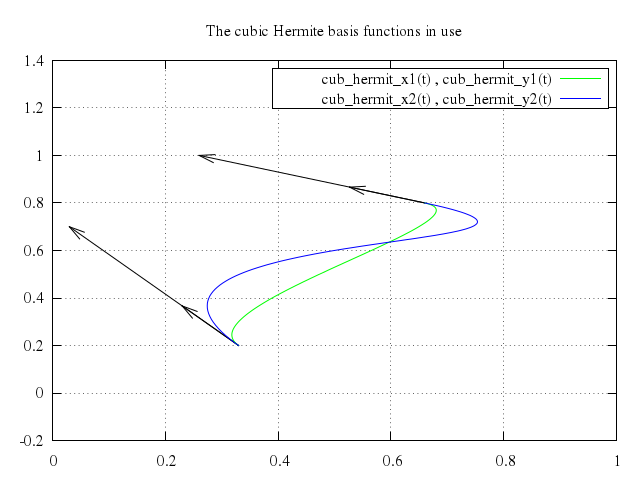
```ruby
# unset arrow
# #
# # Note the arrows here, scaled by 1/3 so they will fit into plotting area
# #
# set arrow from x1,y1 to x1+xv0/3,y1+yv0/3
# set arrow from x2,y2 to x2+xv1/3,y2+yv1/3
# set arrow from x1,y1 to x1+xv0,y1+yv0
# set arrow from x2,y2 to x2+xv1,y2+yv1
#
# cub_hermit_x1(t) = h00(t) * x1 + h01(t) * x2 + h10(t) * xv0 + h11(t) * xv1
# cub_hermit_y1(t) = h00(t) * y1 + h01(t) * y2 + h10(t) * yv0 + h11(t) * yv1
# cub_hermit_x2(t) = h00(t) * x1 + h01(t) * x2 + h10(t) * xv0*3 + h11(t) * xv1*3
# cub_hermit_y2(t) = h00(t) * y1 + h01(t) * y2 + h10(t) * yv0*3 + h11(t) * yv1*3
# set title "The cubic Hermite basis functions in use"
# plot cub_hermit_x1(t), cub_hermit_y1(t) with lines lt 2,\
# cub_hermit_x2(t), cub_hermit_y2(t) with lines lt 3
Numo.gnuplot do
unset :arrow
set :arrow, from:"x1,y1", to:"x1+xv0/3,y1+yv0/3"
set :arrow, from:"x2,y2", to:"x2+xv1/3,y2+yv1/3"
set :arrow, from:"x1,y1", to:"x1+xv0,y1+yv0"
set :arrow, from:"x2,y2", to:"x2+xv1,y2+yv1"
run "cub_hermit_x1(t) = h00(t) * x1 + h01(t) * x2 + h10(t) * xv0 + h11(t) * xv1"
run "cub_hermit_y1(t) = h00(t) * y1 + h01(t) * y2 + h10(t) * yv0 + h11(t) * yv1"
run "cub_hermit_x2(t) = h00(t) * x1 + h01(t) * x2 + h10(t) * xv0*3 + h11(t) * xv1*3"
run "cub_hermit_y2(t) = h00(t) * y1 + h01(t) * y2 + h10(t) * yv0*3 + h11(t) * yv1*3"
set title:"The cubic Hermite basis functions in use"
plot "cub_hermit_x1(t)",
["cub_hermit_y1(t)", with:"lines", lt:2],
"cub_hermit_x2(t)",
["cub_hermit_y2(t)", with:"lines", lt:3]
end
```
## Bezier splines
[Original Demo](http://gnuplot.sourceforge.net/demo_4.6/airfoil.html)
### 1
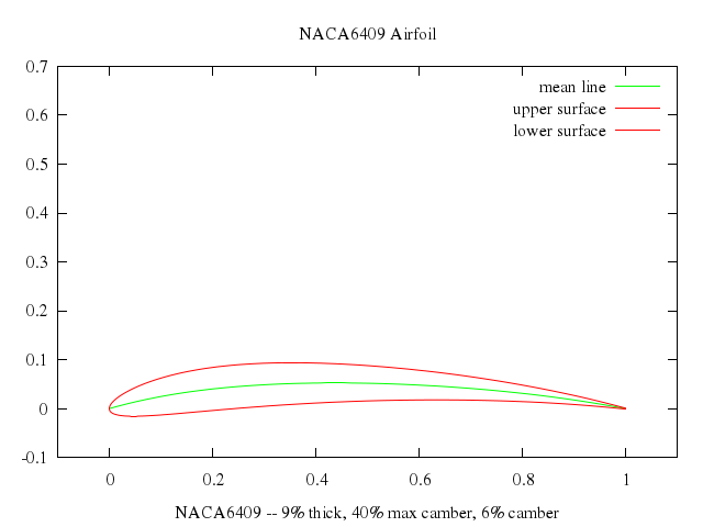
```ruby
# # This demo shows how to use bezier splines to define NACA four
# # series airfoils and complex variables to define Joukowski
# # Airfoils. It will be expanded after overplotting in implemented
# # to plot Coefficient of Pressure as well.
# # Alex Woo, Dec. 1992
# #
# # The definitions below follows: "Bezier presentation of airfoils",
# # by Wolfgang Boehm, Computer Aided Geometric Design 4 (1987) pp 17-22.
# #
# # Gershon Elber, Nov. 1992
# #
# # m = percent camber
# # p = percent chord with maximum camber
# print "NACA four series airfoils by bezier splines"
# print "Will add pressure distribution later with Overplotting"
# mm = 0.6
# # NACA6xxx
# thick = 0.09
# # nine percent NACAxx09
# pp = 0.4
# # NACAx4xx
# # Combined this implies NACA6409 airfoil
# #
# # Airfoil thickness function.
# #
# set xlabel "NACA6409 -- 9% thick, 40% max camber, 6% camber"
# x0 = 0.0
# y0 = 0.0
# x1 = 0.0
# y1 = 0.18556
# x2 = 0.03571
# y2 = 0.34863
# x3 = 0.10714
# y3 = 0.48919
# x4 = 0.21429
# y4 = 0.58214
# x5 = 0.35714
# y5 = 0.55724
# x6 = 0.53571
# y6 = 0.44992
# x7 = 0.75000
# y7 = 0.30281
# x8 = 1.00000
# y8 = 0.01050
# #
# # Directly defining the order 8 Bezier basis function for a faster evaluation.
# #
# bez_d4_i0(x) = (1 - x)**4
# bez_d4_i1(x) = 4 * (1 - x)**3 * x
# bez_d4_i2(x) = 6 * (1 - x)**2 * x**2
# bez_d4_i3(x) = 4 * (1 - x)**1 * x**3
# bez_d4_i4(x) = x**4
#
# bez_d8_i0(x) = (1 - x)**8
# bez_d8_i1(x) = 8 * (1 - x)**7 * x
# bez_d8_i2(x) = 28 * (1 - x)**6 * x**2
# bez_d8_i3(x) = 56 * (1 - x)**5 * x**3
# bez_d8_i4(x) = 70 * (1 - x)**4 * x**4
# bez_d8_i5(x) = 56 * (1 - x)**3 * x**5
# bez_d8_i6(x) = 28 * (1 - x)**2 * x**6
# bez_d8_i7(x) = 8 * (1 - x) * x**7
# bez_d8_i8(x) = x**8
#
# m0 = 0.0
# m1 = 0.1
# m2 = 0.1
# m3 = 0.1
# m4 = 0.0
# mean_y(t) = m0 * mm * bez_d4_i0(t) + \
# m1 * mm * bez_d4_i1(t) + \
# m2 * mm * bez_d4_i2(t) + \
# m3 * mm * bez_d4_i3(t) + \
# m4 * mm * bez_d4_i4(t)
#
# p0 = 0.0
# p1 = pp / 2
# p2 = pp
# p3 = (pp + 1) / 2
# p4 = 1.0
# mean_x(t) = p0 * bez_d4_i0(t) + \
# p1 * bez_d4_i1(t) + \
# p2 * bez_d4_i2(t) + \
# p3 * bez_d4_i3(t) + \
# p4 * bez_d4_i4(t)
#
# z_x(x) = x0 * bez_d8_i0(x) + x1 * bez_d8_i1(x) + x2 * bez_d8_i2(x) + \
# x3 * bez_d8_i3(x) + x4 * bez_d8_i4(x) + x5 * bez_d8_i5(x) + \
# x6 * bez_d8_i6(x) + x7 * bez_d8_i7(x) + x8 * bez_d8_i8(x)
#
# z_y(x, tk) = \
# y0 * tk * bez_d8_i0(x) + y1 * tk * bez_d8_i1(x) + y2 * tk * bez_d8_i2(x) + \
# y3 * tk * bez_d8_i3(x) + y4 * tk * bez_d8_i4(x) + y5 * tk * bez_d8_i5(x) + \
# y6 * tk * bez_d8_i6(x) + y7 * tk * bez_d8_i7(x) + y8 * tk * bez_d8_i8(x)
#
# #
# # Given t value between zero and one, the airfoild curve is defined as
# #
# # c(t) = mean(t1(t)) +/- z(t2(t)) n(t1(t)),
# #
# # where n is the unit normal to the mean line. See the above paper for more.
# #
# # Unfortunately, the parametrization of c(t) is not the same for mean(t1)
# # and z(t2). The mean line (and its normal) can assume linear function t1 = t,
# # -1
# # but the thickness z_y is, in fact, a function of z_x (t). Since it is
# # not obvious how to compute this inverse function analytically, we instead
# # replace t in c(t) equation above by z_x(t) to get:
# #
# # c(z_x(t)) = mean(z_x(t)) +/- z(t) n(z_x(t)),
# #
# # and compute and display this instead. Note we also ignore n(t) and assumes
# # n(t) is constant in the y direction,
# #
#
# airfoil_y1(t, thick) = mean_y(z_x(t)) + z_y(t, thick)
# airfoil_y2(t, thick) = mean_y(z_x(t)) - z_y(t, thick)
# airfoil_y(t) = mean_y(z_x(t))
# airfoil_x(t) = mean_x(z_x(t))
# unset grid
# unset zeroaxis
# set parametric
# set xrange [-0.1:1.1]
# set yrange [-0.1:.7]
# set trange [ 0.0:1.0]
# set title "NACA6409 Airfoil"
# plot airfoil_x(t), airfoil_y(t) title "mean line" w l lt 2, \
# airfoil_x(t), airfoil_y1(t, thick) title "upper surface" w l lt 1, \
# airfoil_x(t), airfoil_y2(t, thick) title "lower surface" w l lt 1
Numo.gnuplot do
run "mm = 0.6"
run "thick = 0.09"
run "pp = 0.4"
set xlabel:"NACA6409 -- 9% thick, 40% max camber, 6% camber"
run "x0 = 0.0"
run "y0 = 0.0"
run "x1 = 0.0"
run "y1 = 0.18556"
run "x2 = 0.03571"
run "y2 = 0.34863"
run "x3 = 0.10714"
run "y3 = 0.48919"
run "x4 = 0.21429"
run "y4 = 0.58214"
run "x5 = 0.35714"
run "y5 = 0.55724"
run "x6 = 0.53571"
run "y6 = 0.44992"
run "x7 = 0.75000"
run "y7 = 0.30281"
run "x8 = 1.00000"
run "y8 = 0.01050"
run "bez_d4_i0(x) = (1 - x)**4"
run "bez_d4_i1(x) = 4 * (1 - x)**3 * x"
run "bez_d4_i2(x) = 6 * (1 - x)**2 * x**2"
run "bez_d4_i3(x) = 4 * (1 - x)**1 * x**3"
run "bez_d4_i4(x) = x**4"
run "bez_d8_i0(x) = (1 - x)**8"
run "bez_d8_i1(x) = 8 * (1 - x)**7 * x"
run "bez_d8_i2(x) = 28 * (1 - x)**6 * x**2"
run "bez_d8_i3(x) = 56 * (1 - x)**5 * x**3"
run "bez_d8_i4(x) = 70 * (1 - x)**4 * x**4"
run "bez_d8_i5(x) = 56 * (1 - x)**3 * x**5"
run "bez_d8_i6(x) = 28 * (1 - x)**2 * x**6"
run "bez_d8_i7(x) = 8 * (1 - x) * x**7"
run "bez_d8_i8(x) = x**8"
run "m0 = 0.0"
run "m1 = 0.1"
run "m2 = 0.1"
run "m3 = 0.1"
run "m4 = 0.0"
run "mean_y(t) = m0 * mm * bez_d4_i0(t) + m1 * mm * bez_d4_i1(t) + m2 * mm * bez_d4_i2(t) + m3 * mm * bez_d4_i3(t) + m4 * mm * bez_d4_i4(t)"
run "p0 = 0.0"
run "p1 = pp / 2"
run "p2 = pp"
run "p3 = (pp + 1) / 2"
run "p4 = 1.0"
run "mean_x(t) = p0 * bez_d4_i0(t) + p1 * bez_d4_i1(t) + p2 * bez_d4_i2(t) + p3 * bez_d4_i3(t) + p4 * bez_d4_i4(t)"
run "z_x(x) = x0 * bez_d8_i0(x) + x1 * bez_d8_i1(x) + x2 * bez_d8_i2(x) + x3 * bez_d8_i3(x) + x4 * bez_d8_i4(x) + x5 * bez_d8_i5(x) + x6 * bez_d8_i6(x) + x7 * bez_d8_i7(x) + x8 * bez_d8_i8(x)"
run "z_y(x, tk) = y0 * tk * bez_d8_i0(x) + y1 * tk * bez_d8_i1(x) + y2 * tk * bez_d8_i2(x) + y3 * tk * bez_d8_i3(x) + y4 * tk * bez_d8_i4(x) + y5 * tk * bez_d8_i5(x) + y6 * tk * bez_d8_i6(x) + y7 * tk * bez_d8_i7(x) + y8 * tk * bez_d8_i8(x)"
run "airfoil_y1(t, thick) = mean_y(z_x(t)) + z_y(t, thick)"
run "airfoil_y2(t, thick) = mean_y(z_x(t)) - z_y(t, thick)"
run "airfoil_y(t) = mean_y(z_x(t))"
run "airfoil_x(t) = mean_x(z_x(t))"
unset :grid
unset :zeroaxis
set :parametric
set xrange:-0.1..1.1
set yrange:-0.1..0.7
set trange:0.0..1.0
set title:"NACA6409 Airfoil"
plot "airfoil_x(t)",
["airfoil_y(t)", title:"mean line", w:"l", lt:2],
"airfoil_x(t)",
["airfoil_y1(t, thick)", title:"upper surface", w:"l", lt:1],
"airfoil_x(t)",
["airfoil_y2(t, thick)", title:"lower surface", w:"l", lt:1]
end
```
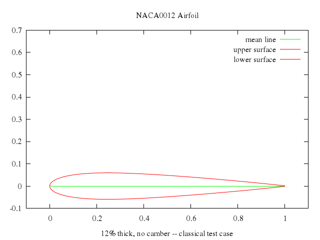
### 2
```ruby
# mm = 0.0
# pp = .5
# thick = .12
# set title "NACA0012 Airfoil"
# set xlabel "12% thick, no camber -- classical test case"
# plot airfoil_x(t), airfoil_y(t) title "mean line" w l lt 2, \
# airfoil_x(t), airfoil_y1(t, thick) title "upper surface" w l lt 1, \
# airfoil_x(t), airfoil_y2(t, thick) title "lower surface" w l lt 1
Numo.gnuplot do
run "mm = 0.0"
run "pp = .5"
run "thick = .12"
set title:"NACA0012 Airfoil"
set xlabel:"12% thick, no camber -- classical test case"
plot "airfoil_x(t)",
["airfoil_y(t)", title:"mean line", w:"l", lt:2],
"airfoil_x(t)",
["airfoil_y1(t, thick)", title:"upper surface", w:"l", lt:1],
"airfoil_x(t)",
["airfoil_y2(t, thick)", title:"lower surface", w:"l", lt:1]
end
```
### 3
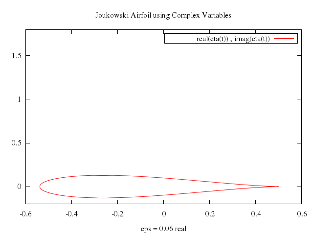
```ruby
# set title ""
# set xlab ""
# set key box
# set parametric
# set samples 100
# set isosamples 10
# set style data lines
# set style function lines
# print "Joukowski Airfoil using Complex Variables"
# set title "Joukowski Airfoil using Complex Variables" offset 0,0
# set time
# set yrange [-.2 : 1.8]
# set trange [0: 2*pi]
# set xrange [-.6:.6]
# zeta(t) = -eps + (a+eps)*exp(t*{0,1})
# eta(t) = zeta(t) + a*a/zeta(t)
# eps = 0.06
# a =.250
# set xlabel "eps = 0.06 real"
# plot real(eta(t)),imag(eta(t))
Numo.gnuplot do
set title:""
set xlab:""
set :key, :box
set :parametric
set samples:100
set isosamples:10
set :style, :data, :lines
set :style, :function, :lines
set title:"Joukowski Airfoil using Complex Variables", offset:[0,0]
#set :time
set yrange:-0.2..1.8
set trange:"[0:2*pi]"
set xrange:-0.6..0.6
run "zeta(t) = -eps + (a+eps)*exp(t*{0,1})"
run "eta(t) = zeta(t) + a*a/zeta(t)"
run "eps = 0.06"
run "a =.250"
set xlabel:"eps = 0.06 real"
plot "real(eta(t))",
"imag(eta(t))"
end
```
### 4
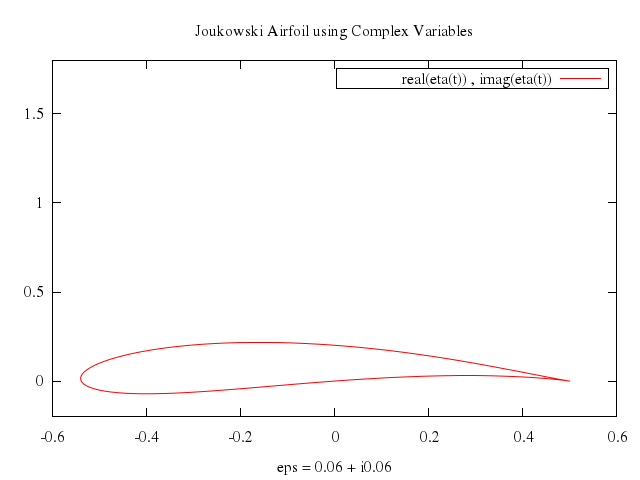
```ruby
# eps = 0.06*{1,-1}
# set xlabel "eps = 0.06 + i0.06"
# plot real(eta(t)),imag(eta(t))
Numo.gnuplot do
run "eps = 0.06*{1,-1}"
set xlabel:"eps = 0.06 + i0.06"
plot "real(eta(t))",
"imag(eta(t))"
end
```
## parameter fitting
[Original Demo](http://gnuplot.sourceforge.net/demo_4.6/fit.html)
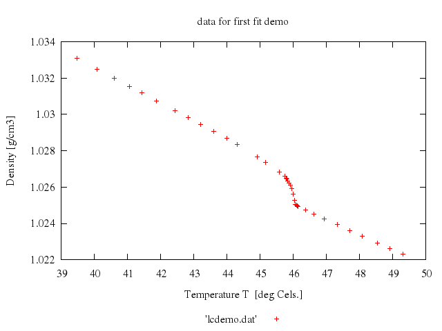
### 1
```ruby
# print "Some examples how data fitting using nonlinear least squares fit"
# print "can be done."
# print ""
#
# reset
# set title 'data for first fit demo'
# set xlabel "Temperature T [deg Cels.]"
# set ylabel "Density [g/cm3]"
# set key below
# plot 'lcdemo.dat'
Numo.gnuplot do
reset
set title:'data for first fit demo'
set xlabel:"Temperature T [deg Cels.]"
set ylabel:"Density [g/cm3]"
set :key, "below"
plot "'lcdemo.dat'"
end
```
### 2
```ruby
# print "now fitting a straight line to the data :-)"
# print "only as a demo without physical meaning"
# load 'line.fnc'
# y0 = 0.0
# m = 0.0
# print "fit function and initial parameters are as follows:"
# print GPFUN_l
# show variables y0
# show variables m
# #show variables
# set title 'all fit params set to 0'
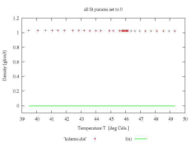
# plot [*:*][-.1:1.2] 'lcdemo.dat', l(x)
Numo.gnuplot do
load 'line.fnc'
run "y0 = 0.0"
run "m = 0.0"
show "variables y0"
show "variables", :m
set title:'all fit params set to 0'
plot "[*:*]", -0.1..1.2,
"'lcdemo.dat'",
"l(x)"
end
```
### 3
```ruby
# print "fit command will be: fit l(x) 'lcdemo.dat' via y0, m"
# fit l(x) 'lcdemo.dat' via y0, m
# set title 'unweighted fit'
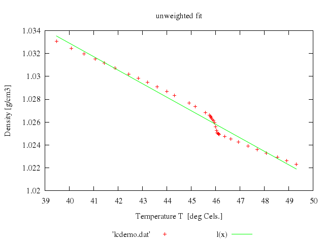
# plot 'lcdemo.dat', l(x)
Numo.gnuplot do
fit 'l(x)', 'lcdemo.dat', via:'y0, m'
set title:'unweighted fit'
plot "'lcdemo.dat'",
"l(x)"
end
```
### 4
```ruby
# print ""
# print "now fit with weights from column 3 which favor low temperatures"
# print "command will be: fit l(x) 'lcdemo.dat' using 1:2:3 via y0, m"
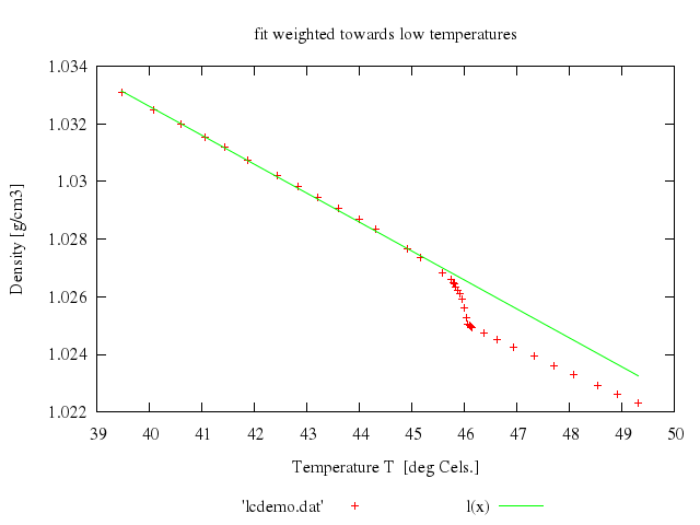
# fit l(x) 'lcdemo.dat' using 1:2:3 via y0, m
# set title 'fit weighted towards low temperatures'
# plot 'lcdemo.dat', l(x)
Numo.gnuplot do
fit 'l(x)', 'lcdemo.dat', using:[1,2,3], via:'y0, m'
set title:'fit weighted towards low temperatures'
plot "'lcdemo.dat'",
"l(x)"
end
```
### 5
```ruby
# print ""
# print "now fit with weights from column 4 instead"
# print "command will be: fit l(x) 'lcdemo.dat' using 1:2:4 via y0, m"
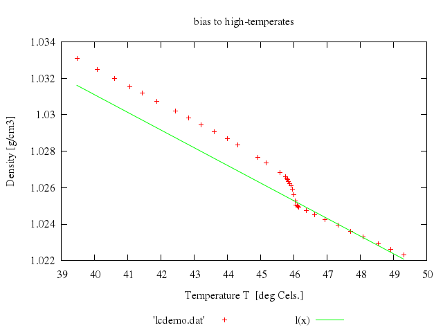
# fit l(x) 'lcdemo.dat' using 1:2:4 via y0, m
# set title 'bias to high-temperates'
# plot 'lcdemo.dat', l(x)
Numo.gnuplot do
fit 'l(x)', 'lcdemo.dat', using:[1,2,4], via:'y0, m'
set title:'bias to high-temperates'
plot "'lcdemo.dat'",
"l(x)"
end
```
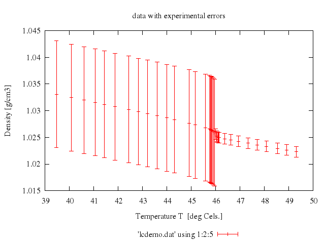
### 6
```ruby
# set title 'data with experimental errors'
# plot 'lcdemo.dat' using 1:2:5 with errorbars
Numo.gnuplot do
set title:'data with experimental errors'
plot "'lcdemo.dat'", using:[1,2,5], with:"errorbars"
end
```
### 7
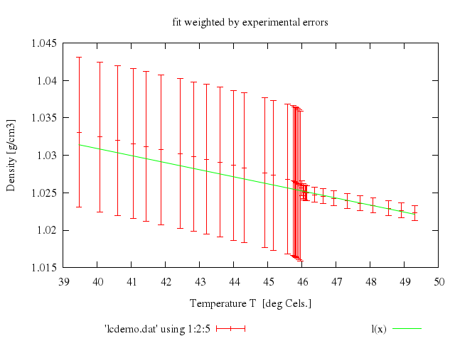
```ruby
# print ""
# print "now use these real single-measurement errors from column 5 to reach "
# print "such a result (look at the file lcdemo.dat and compare the columns to "
# print "see the difference)"
# print "command will be: fit l(x) 'lcdemo.dat' using 1:2:5 via y0, m"
# fit l(x) 'lcdemo.dat' using 1:2:5 via y0, m
# set title 'fit weighted by experimental errors'
# plot 'lcdemo.dat' using 1:2:5 with errorbars, l(x)
Numo.gnuplot do
fit 'l(x)', 'lcdemo.dat', using:[1,2,5], via:'y0, m'
set title:'fit weighted by experimental errors'
plot ["'lcdemo.dat'", using:[1,2,5], with:"errorbars"],
"l(x)"
end
```
### 8
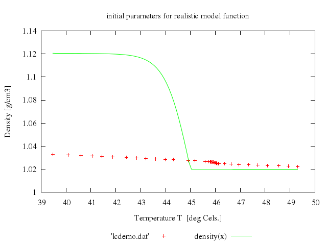
```ruby
# load 'density.fnc'
# set title 'initial parameters for realistic model function'
# plot 'lcdemo.dat', density(x)
Numo.gnuplot do
load 'density.fnc'
set title:'initial parameters for realistic model function'
plot "'lcdemo.dat'",
"density(x)"
end
```
### 9
```ruby
# print ""
# print "It's time now to try a more realistic model function:"
# print GPFUN_density
# print GPFUN_curve
# print GPFUN_lowlin
# print GPFUN_high
# #show functions
# print "density(x) is a function which shall fit the whole temperature"
# print "range using a ?: expression. It contains 6 model parameters which"
# print "will all be varied. Now take the start parameters out of the"
# print "file 'start.par' and plot the function."
# print "command will be: fit density(x) 'lcdemo.dat' via 'start.par'"
# load 'start.par'
# fit density(x) 'lcdemo.dat' via 'start.par'
# set title 'fitted to realistic model function'
# plot 'lcdemo.dat', density(x)
Numo.gnuplot do
load 'start.par'
fit 'density(x)', 'lcdemo.dat', via:"'start.par'"
set title:'fitted to realistic model function'
plot "'lcdemo.dat'",
"density(x)"
end
```

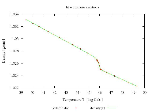
### 10
```ruby
# print ""
# print "looks already rather nice? We will do now the following: set"
# print "the epsilon limit higher so that we need more iteration steps"
# print "to convergence. During fitting please hit ctrl-C. You will be asked"
# print "Stop, Continue, Execute: Try everything. You may define a script"
# print "using the FIT_SCRIPT environment variable. An example would be"
# print "'FIT_SCRIPT=plot nonsense.dat'. Normally you don't need to set"
# print "FIT_SCRIPT since it defaults to 'replot'. Please note that FIT_SCRIPT"
# print "cannot be set from inside gnuplot."
# print ""
# print "command will be: fit density(x) 'lcdemo.dat' via 'start.par'"
# FIT_LIMIT = 1e-10
# fit density(x) 'lcdemo.dat' via 'start.par'
# set title 'fit with more iterations'
# plot 'lcdemo.dat', density(x)
Numo.gnuplot do
run "FIT_LIMIT = 1e-10"
fit 'density(x)', 'lcdemo.dat', via:"'start.par'"
set title:'fit with more iterations'
plot "'lcdemo.dat'",
"density(x)"
end
```
### 11
```ruby
# FIT_LIMIT = 1e-5
# print "\nNow a brief demonstration of 3d fitting."
# print "hemisphr.dat contains random points on a hemisphere of"
# print "radius 1, but we let fit figure this out for us."
# print "It takes many iterations, so we limit FIT_MAXITER to 50."
# #HBB: made this a lot harder: also fit the center of the sphere
# #h(x,y) = sqrt(r*r - (x-x0)**2 - (y-y0)**2) + z0
# #HBB 970522: distort the function, so it won't fit exactly:
# h(x,y) = sqrt(r*r - (abs(x-x0))**2.2 - (abs(y-y0))**1.8) + z0
# x0 = 0.1
# y0 = 0.2
# z0 = 0.3
# r=0.5
# FIT_MAXITER=50
# set title 'the scattered points, and the initial parameter'
# splot 'hemisphr.dat' using 1:2:3, h(x,y)
Numo.gnuplot do
run "FIT_LIMIT = 1e-5"
run "h(x,y) = sqrt(r*r - (abs(x-x0))**2.2 - (abs(y-y0))**1.8) + z0"
run "x0 = 0.1"
run "y0 = 0.2"
run "z0 = 0.3"
run "r=0.5"
run "FIT_MAXITER=50"
set title:'the scattered points, and the initial parameter'
splot ["'hemisphr.dat'", using:[1,2,3]],
"h(x,y)"
end
```
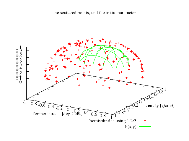
### 12
```ruby
# print "fit function will be: " . GPFUN_h
# print "we *must* provide 4 columns for a 3d fit. We fake errors=1"
# print "command will be: fit h(x,y) 'hemisphr.dat' using 1:2:3:(1) via r, x0,y0,z0"
#
# # we *must* provide 4 columns for a 3d fit. We fake errors=1
# fit h(x,y) 'hemisphr.dat' using 1:2:3:(1) via r, x0, y0, z0
# set title 'the scattered points, fitted curve'
# splot 'hemisphr.dat' using 1:2:3, h(x,y)
Numo.gnuplot do
fit 'h(x,y)', 'hemisphr.dat', using:'1:2:3:(1)', via:'r, x0, y0, z0'
set title:'the scattered points, fitted curve'
splot ["'hemisphr.dat'", using:[1,2,3]],
"h(x,y)"
end
```
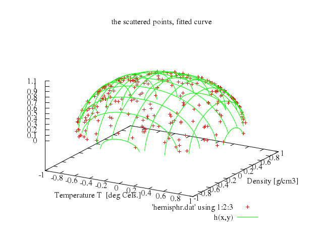
### 13
```ruby
# print "\n\nNotice, however, that this would converge much faster when"
# print "fitted in a more appropriate co-ordinate system:"
# print "fit r 'hemisphr.dat' using 0:($1*$1+$2*$2+$3*$3) via r"
# print "where we are fitting f(x)=r to the radii calculated as the data"
# print "is read from the file. No x value is required in this case."
# FIT_MAXITER=0 # no limit : we cannot delete the variable once set
#
# print "\n\nNow an example how to fit multi-branch functions\n"
# print "The model consists of two branches, the first describing longitudinal"
# print "sound velocity as function of propagation direction (upper data, from "
# print "dataset 1), the second describing transverse sound velocity (lower "
# print "data, from dataset 0).\n"
# print "The model uses these data in order to fit elastic stiffnesses"
# print "which occur differently in both branches."
# load 'hexa.fnc'
# load 'sound.par'
# set title 'sound data, and model with initial parameters'
# plot 'soundvel.dat', vlong(x), vtrans(x)
Numo.gnuplot do
run "FIT_MAXITER=0 # no limit : we cannot delete the variable once set"
load 'hexa.fnc'
load 'sound.par'
set title:'sound data, and model with initial parameters'
plot "'soundvel.dat'",
"vlong(x)",
"vtrans(x)"
end
```
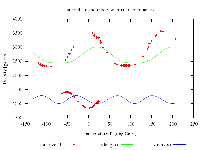
### 14
```ruby
# print ""
# print "fit function will be: " . GPFUN_f
# print GPFUN_vlong
# print GPFUN_vtrans
# print "y will be the index of the dataset"
# print "command will be: fit f(x,y) 'soundvel.dat' using 1:-2:2:(1) via 'sound.par'"
# # Must provide an error estimate for a 3d fit. Use constant 1
# fit f(x,y) 'soundvel.dat' using 1:-2:2:(1) via 'sound.par'
# #create soundfit.par, reading from sound.par and updating values
# update 'sound.par' 'soundfit.par'
# print ""
# set title 'pseudo-3d multi-branch fit to velocity data'
# plot 'soundvel.dat', vlong(x), vtrans(x)
Numo.gnuplot do
fit 'f(x,y)', 'soundvel.dat', using:'1:-2:2:(1)', via:"'sound.par'"
update 'sound.par', 'soundfit.par'
set title:'pseudo-3d multi-branch fit to velocity data'
plot "'soundvel.dat'",
"vlong(x)",
"vtrans(x)"
end
```
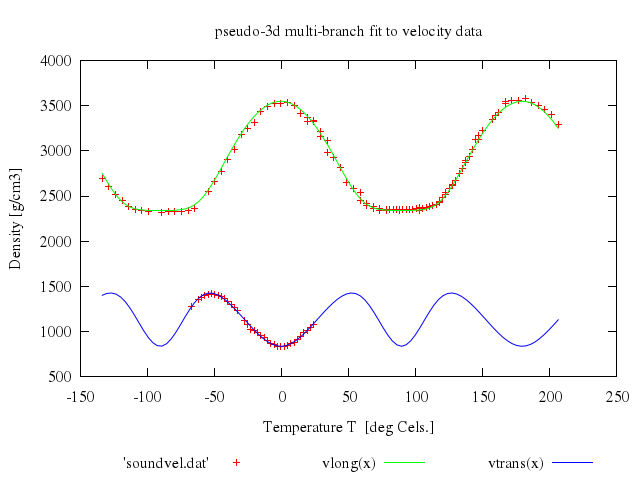
### 15
```ruby
# print "Look at the file 'hexa.fnc' to see how the branches are realized"
# print "using the data index as a pseudo-3d fit"
# print ""
# print "Next we only use every fifth data point for fitting by using the"
# print "'every' keyword. Look at the fitting-speed increase and at"
# print "fitting result."
# print "command will be: fit f(x,y) 'soundvel.dat' every 5 using 1:-2:2:(1) via 'sound.par'"
# load 'sound.par'
# fit f(x,y) 'soundvel.dat' every 5 using 1:-2:2:(1) via 'sound.par'
# set title 'fitted only every 5th data point'
# plot 'soundvel.dat', vlong(x), vtrans(x)
Numo.gnuplot do
load 'sound.par'
fit 'f(x,y)', 'soundvel.dat', every:5, using:'1:-2:2:(1)', via:"'sound.par'"
set title:'fitted only every 5th data point'
plot "'soundvel.dat'",
"vlong(x)",
"vtrans(x)"
end
```
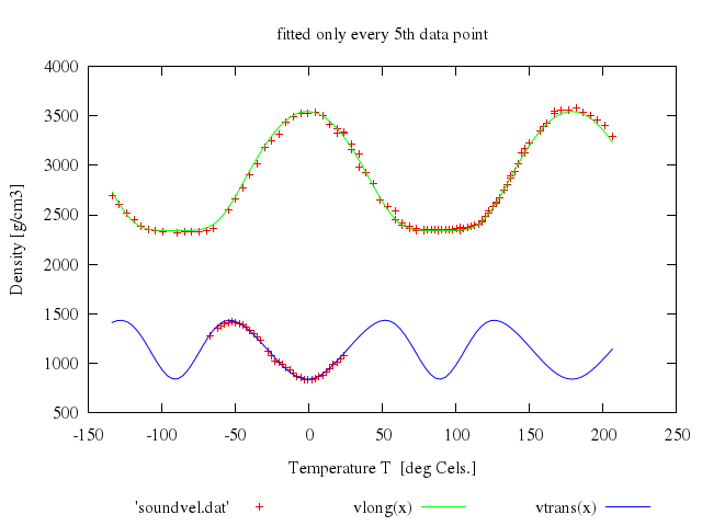
### 16
```ruby
# print "When you compare the results (see 'fit.log') you remark that"
# print "the uncertainties in the fitted constants have become larger,"
# print "the quality of the plot is only slightly affected."
# print ""
# print "By marking some parameters as '# FIXED' in the parameter file"
# print "you fit only the others (c44 and c13 fixed here)."
# print ""
# load 'sound2.par'
# set title 'initial parameters'
# plot 'soundvel.dat', vlong(x), vtrans(x)
Numo.gnuplot do
load 'sound2.par'
set title:'initial parameters'
plot "'soundvel.dat'",
"vlong(x)",
"vtrans(x)"
end
```
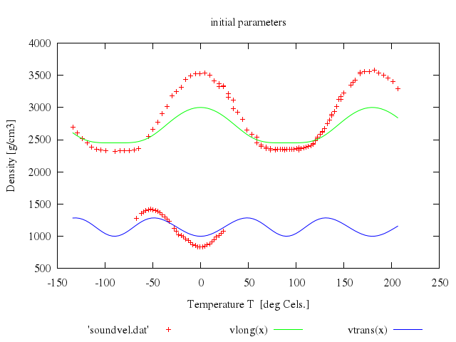
### 17
```ruby
# fit f(x,y) 'soundvel.dat' using 1:-2:2:(1) via 'sound2.par'
# set title 'fit with c44 and c13 fixed'
# plot 'soundvel.dat', vlong(x), vtrans(x)
Numo.gnuplot do
fit 'f(x,y)', 'soundvel.dat', using:'1:-2:2:(1)', via:"'sound2.par'"
set title:'fit with c44 and c13 fixed'
plot "'soundvel.dat'",
"vlong(x)",
"vtrans(x)"
end
```

### 18
```ruby
# print "This has the same effect as specifying only the real free"
# print "parameters by the 'via' syntax."
# print ""
# print "fit f(x) 'soundvel.dat' via c33, c11, phi0"
# print ""
# load 'sound.par'
# set title 'initial parameters'
# plot 'soundvel.dat', vlong(x), vtrans(x)
Numo.gnuplot do
load 'sound.par'
set title:'initial parameters'
plot "'soundvel.dat'",
"vlong(x)",
"vtrans(x)"
end
```
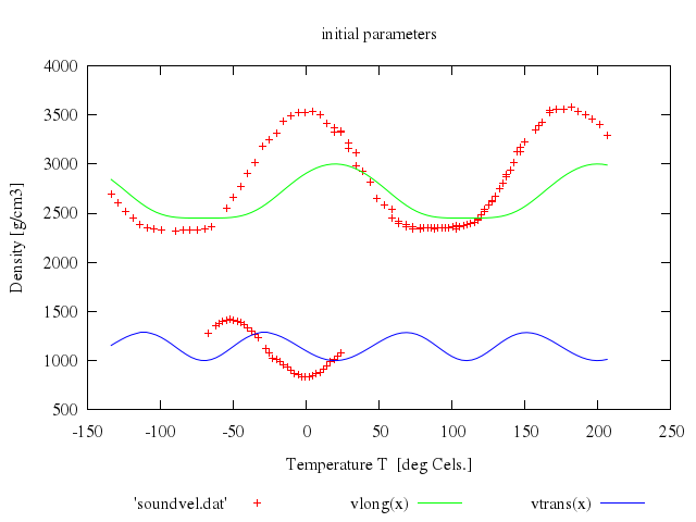
### 19
```ruby
# fit f(x,y) 'soundvel.dat' using 1:-2:2:(1) via c33, c11, phi0
# set title 'fit via c33,c11,phi0'
# plot 'soundvel.dat', vlong(x), vtrans(x)
Numo.gnuplot do
fit 'f(x,y)', 'soundvel.dat', using:'1:-2:2:(1)', via:'c33, c11, phi0'
set title:'fit via c33,c11,phi0'
plot "'soundvel.dat'",
"vlong(x)",
"vtrans(x)"
end
```
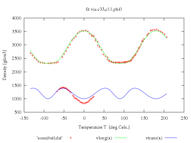
### 20
```ruby
# print "Here comes an example of a very complex function..."
# print ""
#
# set xlabel "Delta [degrees]"
# set ylabel "Reflectivity"
# set title 'raw data'
# #HBB 970522: here and below, use the error column present in moli3.dat:
# plot 'moli3.dat' w e
Numo.gnuplot do
set xlabel:"Delta [degrees]"
set ylabel:"Reflectivity"
set title:'raw data'
plot "'moli3.dat'", w:"e"
end
```
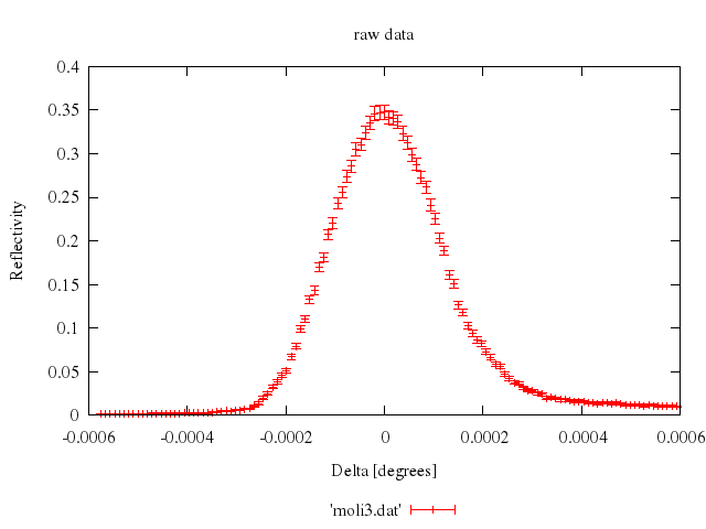
### 21
```ruby
# print "now fitting the model function to the data"
# load 'reflect.fnc'
#
# #HBB 970522: Changed initial values to something sensible, i.e.
# # something an experienced user of fit would actually use.
# # FIT_LIMIT is also raised, to ensure a better fit.
# eta = 1.2e-4
# tc = 1.8e-3
# FIT_LIMIT=1e-10
#
# #show variables
# #show functions
# set title 'initial parameters'
# plot 'moli3.dat' w e, R(x)
Numo.gnuplot do
load 'reflect.fnc'
run "eta = 1.2e-4"
run "tc = 1.8e-3"
run "FIT_LIMIT=1e-10"
set title:'initial parameters'
plot ["'moli3.dat'", w:"e"],
"R(x)"
end
```
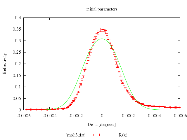
### 22
```ruby
# print "fit function is: " . GPFUN_R
# print GPFUN_a
# print GPFUN_W
# print "command will be: fit R(x) 'moli3.dat' u 1:2:3 via eta, tc"
# fit R(x) 'moli3.dat' u 1:2:3 via eta, tc
# set title 'fitted parameters'
# replot
Numo.gnuplot do
fit 'R(x)', 'moli3.dat', u:[1,2,3], via:'eta, tc'
set title:'fitted parameters'
replot
end
```

### 23
```ruby
# #HBB 970522: added comment on result of last fit.
# print "Looking at the plot of the resulting fit curve, you can see"
# print "that this function doesn't really fit this set of data points."
# print "This would normally be a reason to check for measurement problems"
# print "not yet accounted for, and maybe even re-think the theoretic"
# print "prediction in use."
# print ""
#
# reset
# set xlabel 'x'
# set ylabel 'y'
# set zlabel 'z'
# set ticslevel .2
# set zrange [-3:3]
# splot 'fit3.dat' index 0 using 1:2:4
Numo.gnuplot do
reset
set xlabel:'x'
set ylabel:'y'
set zlabel:'z'
set ticslevel:0.2
set zrange:-3..3
splot "'fit3.dat'", index:0, using:[1,2,4]
end
```
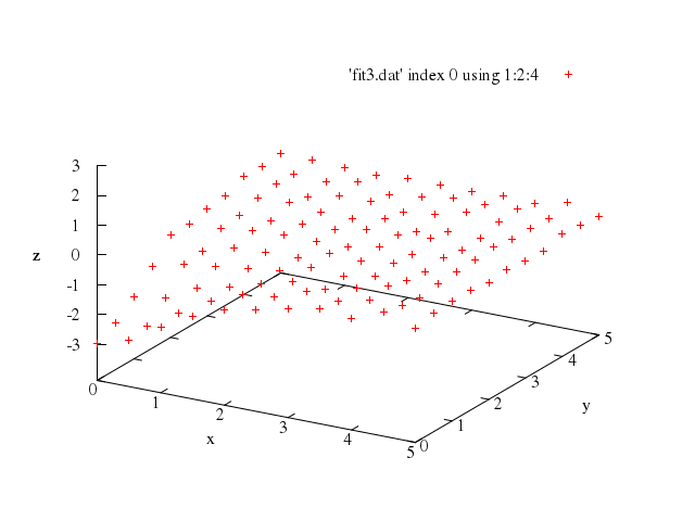
### 24
```ruby
# print ''
# print 'Next we show a fit with three independent variables. The file'
# print 'fit3.dat has four columns, with values of the three independent'
# print 'variable x, y, and t, and the resulting value z. The data'
# print 'lines are in four sections, with t being constant within each'
# print 'section. The sections are separated by two blank lines, so we'
# print 'can select sections with "index" modifiers. Here are the data in'
# print 'the first section, where t = -3.'
# print ''
# print 'We will fit the function a0/(1 + a1*x**2 + a2*y**2) to these'
# print 'data. Since at this point we have two independent variables,'
# print 'our "using" spec has four entries, representing x:y:z:s (where'
# print 's is the estimated error in the z value).'
#
# print "Command will be: "
# print " fit a0/(1+a1*x**2+a2*y**2) 'fit3.dat' index 0 using 1:2:4:(1) via a0,a1,a2"
# a0=1; a1=.1; a2=.1
# fit a0/(1+a1*x**2+a2*y**2) 'fit3.dat' index 0 using 1:2:4:(1) via a0,a1,a2
# splot a0/(1+a1*x**2+a2*y**2), 'fit3.dat' in 0 u 1:2:4
Numo.gnuplot do
run "a0=1; a1=.1; a2=.1"
fit 'a0/(1+a1*x**2+a2*y**2)', 'fit3.dat', index:0, using:'1:2:4:(1)', via:'a0,a1,a2'
splot "a0/(1+a1*x**2+a2*y**2)",
["'fit3.dat'", in:0, u:[1,2,4]]
end
```
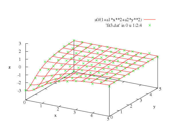
### 25
```ruby
# splot a0/(1+a1*x**2+a2*y**2), 'fit3.dat' in 3 u 1:2:4
Numo.gnuplot do
splot "a0/(1+a1*x**2+a2*y**2)",
["'fit3.dat'", in:3, u:[1,2,4]]
end
```
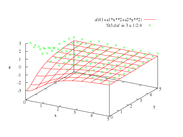
### 26
```ruby
# print ""
# print "Here is the last set of data where t = 3."
# print "We fit the same function to this set."
# print "Command will be: "
# print " fit a0/(1+a1*x**2+a2*y**2) 'fit3.dat' in 3 u 1:2:4:(1) via a0,a1,a2"
# fit a0/(1+a1*x**2+a2*y**2) 'fit3.dat' in 3 u 1:2:4:(1) via a0,a1,a2
# splot a0/(1+a1*x**2+a2*y**2), 'fit3.dat' in 3 u 1:2:4
Numo.gnuplot do
fit 'a0/(1+a1*x**2+a2*y**2)', 'fit3.dat', in:3, u:'1:2:4:(1)', via:'a0,a1,a2'
splot "a0/(1+a1*x**2+a2*y**2)",
["'fit3.dat'", in:3, u:[1,2,4]]
end
```
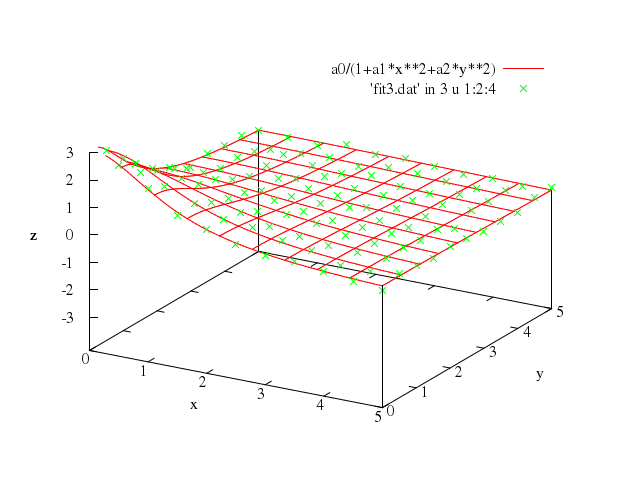
### 27
```ruby
# splot a0/(1+a1*x**2+a2*y**2), 'fit3.dat' u 1:2:4
Numo.gnuplot do
splot "a0/(1+a1*x**2+a2*y**2)",
["'fit3.dat'", u:[1,2,4]]
end
```
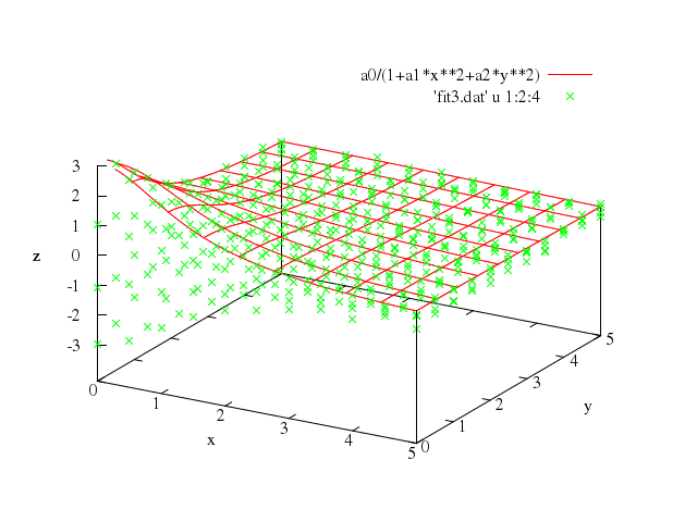
### 28
```ruby
# print ""
# print "We also have data for several intermediate values of t. We"
# print "will fit the function f(x,y,t)=a0*t/(1+a1*x**2+a2*y**2) to all"
# print "the data. Since there are now three independent variables, we"
# print "need a using spec with five entries, representing x:y:t:z:s."
# print "Command will be: "
# print " fit f(x,y,t) 'fit3.dat' u 1:2:3:4:(1) via a0,a1,a2"
# f(x,y,t)=a0*t/(1+a1*x**2+a2*y**2)
# fit f(x,y,t) 'fit3.dat' u 1:2:3:4:(1) via a0,a1,a2
#
# print "We plot the data in each section with the corresponding"
# print "function values."
#
# splot f(x,y,-3), 'fit3.dat' in 0 u 1:2:4
Numo.gnuplot do
run "f(x,y,t)=a0*t/(1+a1*x**2+a2*y**2)"
fit 'f(x,y,t)', 'fit3.dat', u:'1:2:3:4:(1)', via:'a0,a1,a2'
splot "f(x,y,-3)",
["'fit3.dat'", in:0, u:[1,2,4]]
end
```
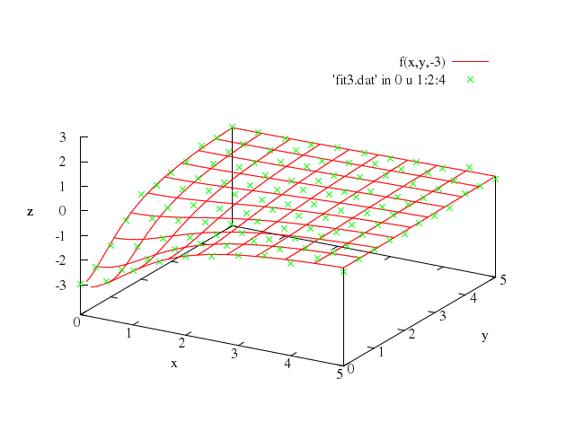
### 29
```ruby
# splot f(x,y,-1), 'fit3.dat' in 1 u 1:2:4
Numo.gnuplot do
splot "f(x,y,-1)",
["'fit3.dat'", in:1, u:[1,2,4]]
end
```
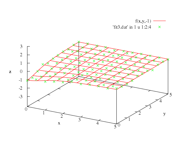
### 30
```ruby
# splot f(x,y,1), 'fit3.dat' in 2 u 1:2:4
Numo.gnuplot do
splot "f(x,y,1)",
["'fit3.dat'", in:2, u:[1,2,4]]
end
```
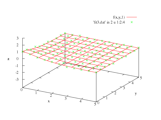
### 31
```ruby
# splot f(x,y,3), 'fit3.dat' in 3 u 1:2:4
Numo.gnuplot do
splot "f(x,y,3)",
["'fit3.dat'", in:3, u:[1,2,4]]
end
```
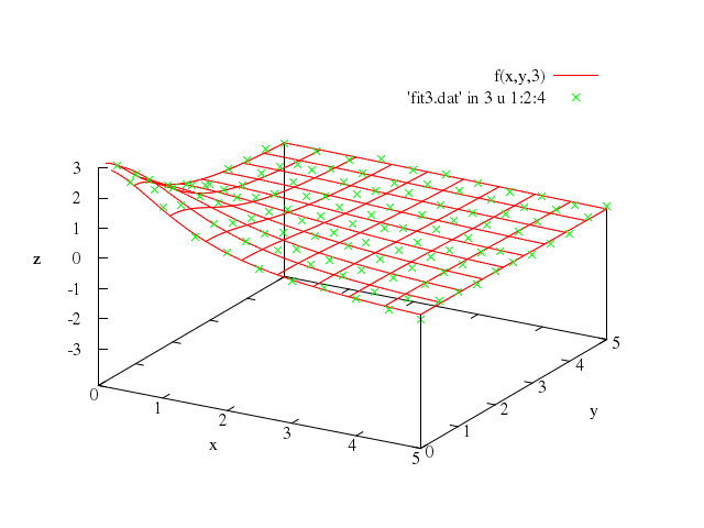
### 32
```ruby
# splot f(x,y,3), 'fit3.dat' in 3 u 1:2:4, \
# f(x,y,1), 'fit3.dat' in 2 u 1:2:4, \
# f(x,y,-1), 'fit3.dat' in 1 u 1:2:4, \
# f(x,y,-3), 'fit3.dat' in 0 u 1:2:4
Numo.gnuplot do
splot "f(x,y,3)",
["'fit3.dat'", in:3, u:[1,2,4]],
"f(x,y,1)",
["'fit3.dat'", in:2, u:[1,2,4]],
"f(x,y,-1)",
["'fit3.dat'", in:1, u:[1,2,4]],
"f(x,y,-3)",
["'fit3.dat'", in:0, u:[1,2,4]]
end
```
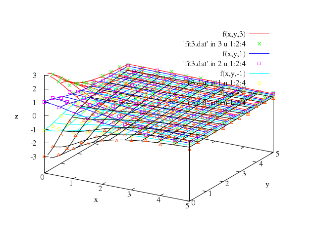
## probability
[Original Demo](http://gnuplot.sourceforge.net/demo_4.6/prob2.html)
### 1
```ruby
# # Demo Statistical Approximations version 1.1
# #
# # Copyright (c) 1991, Jos van der Woude, [email protected]
#
# # History:
# # -- --- 1991 Jos van der Woude: 1st version
# # 06 Jun 2006 Dan Sebald: Added plot methods for better visual effect.
#
# print ""
# print " Statistical Approximations, version 1.1"
# print ""
# print " Copyright (c) 1991, 1992, Jos van de Woude, [email protected]"
# print ""
# print " NOTE: contains 10 plots and consequently takes some time to run"
# print " Press Ctrl-C to exit right now"
# print ""
#
# load "stat.inc"
# rnd(x) = floor(x+0.5)
# r_xmin = -1
# r_sigma = 4.0
#
# # Binomial PDF using normal approximation
# n = 25; p = 0.15
# mu = n * p
# sigma = sqrt(n * p * (1.0 - p))
# xmin = floor(mu - r_sigma * sigma)
# xmin = xmin < r_xmin ? r_xmin : xmin
# xmax = ceil(mu + r_sigma * sigma)
# ymax = 1.1 * binom(floor((n+1)*p), n, p) #mode of binomial PDF used
# set key box
# unset zeroaxis
# set xrange [xmin - 1 : xmax + 1]
# set yrange [0 : ymax]
# set xlabel "k, x ->"
# set ylabel "probability density ->"
# set ytics 0, ymax / 10.0, ymax
# set format x "%2.0f"
# set format y "%3.2f"
# set sample 200
# set title "binomial PDF using normal approximation"
# set arrow from mu, 0 to mu, normal(mu, mu, sigma) nohead
# set arrow from mu, normal(mu + sigma, mu, sigma) \
# to mu + sigma, normal(mu + sigma, mu, sigma) nohead
# set label "mu" at mu + 0.5, ymax / 10
# set label "sigma" at mu + 0.5 + sigma, normal(mu + sigma, mu, sigma)
# plot binom(rnd(x), n, p) with histeps, normal(x, mu, sigma)
Numo.gnuplot do
load "stat.inc"
run "rnd(x) = floor(x+0.5)"
run "r_xmin = -1"
run "r_sigma = 4.0"
run "n = 25; p = 0.15"
run "mu = n * p"
run "sigma = sqrt(n * p * (1.0 - p))"
run "xmin = floor(mu - r_sigma * sigma)"
run "xmin = xmin < r_xmin ? r_xmin : xmin"
run "xmax = ceil(mu + r_sigma * sigma)"
run "ymax = 1.1 * binom(floor((n+1)*p), n, p) #mode of binomial PDF used"
set :key, :box
unset :zeroaxis
set xrange:"[xmin-1:xmax+1]"
set yrange:"[0:ymax]"
set xlabel:"k, x ->"
set ylabel:"probability density ->"
set ytics:'0,ymax/10.0,ymax'
set format_x:"%2.0f"
set format_y:"%3.2f"
set sample:200
set title:"binomial PDF using normal approximation"
set :arrow, from:"mu, 0", to:"mu, normal(mu, mu, sigma)", nohead:true
set :arrow, from:"mu, normal(mu + sigma, mu, sigma)", to:"mu + sigma, normal(mu + sigma, mu, sigma)", nohead:true
set label:"mu", at:"mu + 0.5, ymax / 10"
set label:"sigma", at:"mu + 0.5 + sigma, normal(mu + sigma, mu, sigma)"
plot ["binom(rnd(x), n, p)", with:"histeps"],
"normal(x, mu, sigma)"
end
```
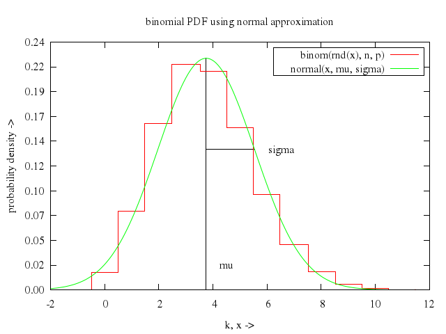
### 2
```ruby
# unset arrow
# unset label
#
# # Binomial PDF using poisson approximation
# n = 50; p = 0.1
# mu = n * p
# sigma = sqrt(mu)
# xmin = floor(mu - r_sigma * sigma)
# xmin = xmin < r_xmin ? r_xmin : xmin
# xmax = ceil(mu + r_sigma * sigma)
# ymax = 1.1 * binom(floor((n+1)*p), n, p) #mode of binomial PDF used
# set key box
# unset zeroaxis
# set xrange [xmin - 1 : xmax + 1]
# set yrange [0 : ymax]
# set xlabel "k ->"
# set ylabel "probability density ->"
# set ytics 0, ymax / 10.0, ymax
# set format x "%2.0f"
# set format y "%3.2f"
# set sample (xmax - xmin + 3)
# set title "binomial PDF using poisson approximation"
# set arrow from mu, 0 to mu, normal(mu, mu, sigma) nohead
# set arrow from mu, normal(mu + sigma, mu, sigma) \
# to mu + sigma, normal(mu + sigma, mu, sigma) nohead
# set label "mu" at mu + 0.5, ymax / 10
# set label "sigma" at mu + 0.5 + sigma, normal(mu + sigma, mu, sigma)
# plot binom(x, n, p) with histeps, poisson(x, mu) with histeps
Numo.gnuplot do
unset :arrow
unset :label
run "n = 50; p = 0.1"
run "mu = n * p"
run "sigma = sqrt(mu)"
run "xmin = floor(mu - r_sigma * sigma)"
run "xmin = xmin < r_xmin ? r_xmin : xmin"
run "xmax = ceil(mu + r_sigma * sigma)"
run "ymax = 1.1 * binom(floor((n+1)*p), n, p) #mode of binomial PDF used"
set :key, :box
unset :zeroaxis
set xrange:"[xmin-1:xmax+1]"
set yrange:"[0:ymax]"
set xlabel:"k ->"
set ylabel:"probability density ->"
set ytics:'0,ymax/10.0,ymax'
set format_x:"%2.0f"
set format_y:"%3.2f"
set sample:'(xmax - xmin + 3)'
set title:"binomial PDF using poisson approximation"
set :arrow, from:"mu, 0", to:"mu, normal(mu, mu, sigma)", nohead:true
set :arrow, from:"mu, normal(mu + sigma, mu, sigma)", to:"mu + sigma, normal(mu + sigma, mu, sigma)", nohead:true
set label:"mu", at:"mu + 0.5, ymax / 10"
set label:"sigma", at:"mu + 0.5 + sigma, normal(mu + sigma, mu, sigma)"
plot ["binom(x, n, p)", with:"histeps"],
["poisson(x, mu)", with:"histeps"]
end
```
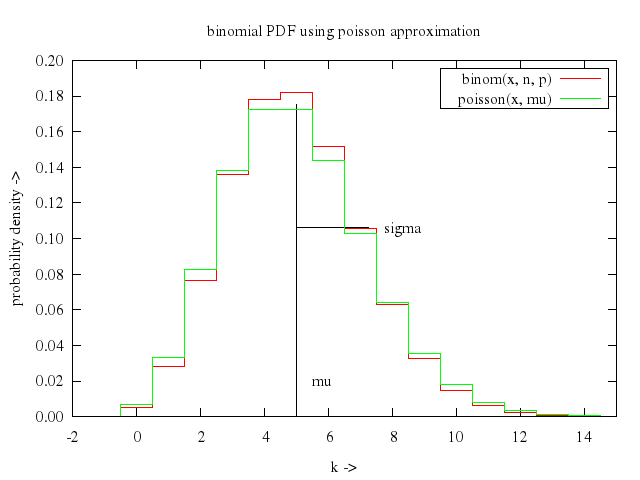
### 3
```ruby
# unset arrow
# unset label
#
# # Geometric PDF using gamma approximation
# p = 0.3
# mu = (1.0 - p) / p
# sigma = sqrt(mu / p)
# lambda = p
# rho = 1.0 - p
# xmin = floor(mu - r_sigma * sigma)
# xmin = xmin < r_xmin ? r_xmin : xmin
# xmax = ceil(mu + r_sigma * sigma)
# ymax = 1.1 * p
# set key box
# unset zeroaxis
# set xrange [xmin - 1 : xmax + 1]
# set yrange [0 : ymax]
# set xlabel "k, x ->"
# set ylabel "probability density ->"
# set ytics 0, ymax / 10.0, ymax
# set format x "%2.0f"
# set format y "%3.2f"
# set sample 200
# set title "geometric PDF using gamma approximation"
# set arrow from mu, 0 to mu, gmm(mu, rho, lambda) nohead
# set arrow from mu, gmm(mu + sigma, rho, lambda) \
# to mu + sigma, gmm(mu + sigma, rho, lambda) nohead
# set label "mu" at mu + 0.5, ymax / 10
# set label "sigma" at mu + 0.5 + sigma, gmm(mu + sigma, rho, lambda)
# plot geometric(rnd(x),p) with histeps, gmm(x, rho, lambda)
Numo.gnuplot do
unset :arrow
unset :label
run "p = 0.3"
run "mu = (1.0 - p) / p"
run "sigma = sqrt(mu / p)"
run "lambda = p"
run "rho = 1.0 - p"
run "xmin = floor(mu - r_sigma * sigma)"
run "xmin = xmin < r_xmin ? r_xmin : xmin"
run "xmax = ceil(mu + r_sigma * sigma)"
run "ymax = 1.1 * p"
set :key, :box
unset :zeroaxis
set xrange:"[xmin-1:xmax+1]"
set yrange:"[0:ymax]"
set xlabel:"k, x ->"
set ylabel:"probability density ->"
set ytics:'0,ymax/10.0,ymax'
set format_x:"%2.0f"
set format_y:"%3.2f"
set sample:200
set title:"geometric PDF using gamma approximation"
set :arrow, from:"mu, 0", to:"mu, gmm(mu, rho, lambda)", nohead:true
set :arrow, from:"mu, gmm(mu + sigma, rho, lambda)", to:"mu + sigma, gmm(mu + sigma, rho, lambda)", nohead:true
set label:"mu", at:"mu + 0.5, ymax / 10"
set label:"sigma", at:"mu + 0.5 + sigma, gmm(mu + sigma, rho, lambda)"
plot ["geometric(rnd(x),p)", with:"histeps"],
"gmm(x, rho, lambda)"
end
```
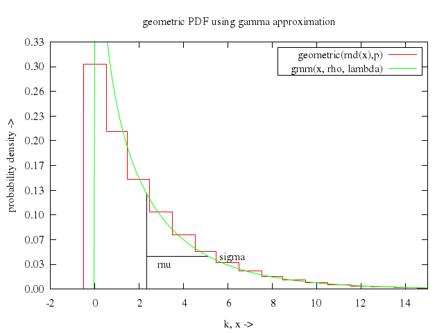
### 4
```ruby
# unset arrow
# unset label
#
# # Geometric PDF using normal approximation
# p = 0.3
# mu = (1.0 - p) / p
# sigma = sqrt(mu / p)
# xmin = floor(mu - r_sigma * sigma)
# xmin = xmin < r_xmin ? r_xmin : xmin
# xmax = ceil(mu + r_sigma * sigma)
# ymax = 1.1 * p
# set key box
# unset zeroaxis
# set xrange [xmin - 1 : xmax + 1]
# set yrange [0 : ymax]
# set xlabel "k, x ->"
# set ylabel "probability density ->"
# set ytics 0, ymax / 10.0, ymax
# set format x "%2.0f"
# set format y "%3.2f"
# set sample 200
# set title "geometric PDF using normal approximation"
# set arrow from mu, 0 to mu, normal(mu, mu, sigma) nohead
# set arrow from mu, normal(mu + sigma, mu, sigma) \
# to mu + sigma, normal(mu + sigma, mu, sigma) nohead
# set label "mu" at mu + 0.5, ymax / 10
# set label "sigma" at mu + 0.5 + sigma, normal(mu + sigma, mu, sigma)
# plot geometric(rnd(x),p) with histeps, normal(x, mu, sigma)
Numo.gnuplot do
unset :arrow
unset :label
run "p = 0.3"
run "mu = (1.0 - p) / p"
run "sigma = sqrt(mu / p)"
run "xmin = floor(mu - r_sigma * sigma)"
run "xmin = xmin < r_xmin ? r_xmin : xmin"
run "xmax = ceil(mu + r_sigma * sigma)"
run "ymax = 1.1 * p"
set :key, :box
unset :zeroaxis
set xrange:"[xmin-1:xmax+1]"
set yrange:"[0:ymax]"
set xlabel:"k, x ->"
set ylabel:"probability density ->"
set ytics:'0,ymax/10.0,ymax'
set format_x:"%2.0f"
set format_y:"%3.2f"
set sample:200
set title:"geometric PDF using normal approximation"
set :arrow, from:"mu, 0", to:"mu, normal(mu, mu, sigma)", nohead:true
set :arrow, from:"mu, normal(mu + sigma, mu, sigma)", to:"mu + sigma, normal(mu + sigma, mu, sigma)", nohead:true
set label:"mu", at:"mu + 0.5, ymax / 10"
set label:"sigma", at:"mu + 0.5 + sigma, normal(mu + sigma, mu, sigma)"
plot ["geometric(rnd(x),p)", with:"histeps"],
"normal(x, mu, sigma)"
end
```
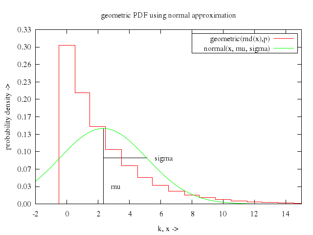
### 5
```ruby
# unset arrow
# unset label
#
# # Hypergeometric PDF using binomial approximation
# nn = 75; mm = 25; n = 10
# p = real(mm) / nn
# mu = n * p
# sigma = sqrt(real(nn - n) / (nn - 1.0) * n * p * (1.0 - p))
# xmin = floor(mu - r_sigma * sigma)
# xmin = xmin < r_xmin ? r_xmin : xmin
# xmax = ceil(mu + r_sigma * sigma)
# ymax = 1.1 * hypgeo(floor(mu), nn, mm, n) #mode of binom PDF used
# set key box
# unset zeroaxis
# set xrange [xmin - 1 : xmax + 1]
# set yrange [0 : ymax]
# set xlabel "k ->"
# set ylabel "probability density ->"
# set ytics 0, ymax / 10.0, ymax
# set format x "%2.0f"
# set format y "%3.2f"
# set sample (xmax - xmin + 3)
# set title "hypergeometric PDF using binomial approximation"
# set arrow from mu, 0 to mu, binom(floor(mu), n, p) nohead
# set arrow from mu, binom(floor(mu + sigma), n, p) \
# to mu + sigma, binom(floor(mu + sigma), n, p) nohead
# set label "mu" at mu + 0.5, ymax / 10
# set label "sigma" at mu + 0.5 + sigma, binom(floor(mu + sigma), n, p)
# plot hypgeo(x, nn, mm, n) with histeps, binom(x, n, p) with histeps
Numo.gnuplot do
unset :arrow
unset :label
run "nn = 75; mm = 25; n = 10"
run "p = real(mm) / nn"
run "mu = n * p"
run "sigma = sqrt(real(nn - n) / (nn - 1.0) * n * p * (1.0 - p))"
run "xmin = floor(mu - r_sigma * sigma)"
run "xmin = xmin < r_xmin ? r_xmin : xmin"
run "xmax = ceil(mu + r_sigma * sigma)"
run "ymax = 1.1 * hypgeo(floor(mu), nn, mm, n) #mode of binom PDF used"
set :key, :box
unset :zeroaxis
set xrange:"[xmin-1:xmax+1]"
set yrange:"[0:ymax]"
set xlabel:"k ->"
set ylabel:"probability density ->"
set ytics:'0,ymax/10.0,ymax'
set format_x:"%2.0f"
set format_y:"%3.2f"
set sample:'(xmax - xmin + 3)'
set title:"hypergeometric PDF using binomial approximation"
set :arrow, from:"mu, 0", to:"mu, binom(floor(mu), n, p)", nohead:true
set :arrow, from:"mu, binom(floor(mu + sigma), n, p)", to:"mu + sigma, binom(floor(mu + sigma), n, p)", nohead:true
set label:"mu", at:"mu + 0.5, ymax / 10"
set label:"sigma", at:"mu + 0.5 + sigma, binom(floor(mu + sigma), n, p)"
plot ["hypgeo(x, nn, mm, n)", with:"histeps"],
["binom(x, n, p)", with:"histeps"]
end
```
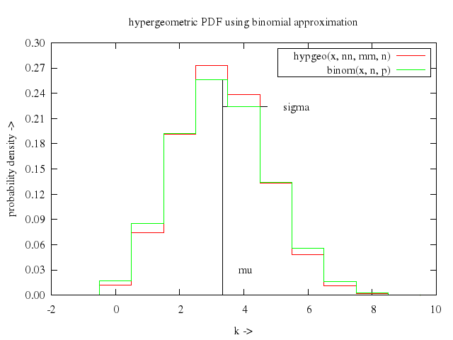
### 6
```ruby
# unset arrow
# unset label
#
# # Hypergeometric PDF using normal approximation
# nn = 75; mm = 25; n = 10
# p = real(mm) / nn
# mu = n * p
# sigma = sqrt(real(nn - n) / (nn - 1.0) * n * p * (1.0 - p))
# xmin = floor(mu - r_sigma * sigma)
# xmin = xmin < r_xmin ? r_xmin : xmin
# xmax = ceil(mu + r_sigma * sigma)
# ymax = 1.1 * hypgeo(floor(mu), nn, mm, n) #mode of binom PDF used
# set key box
# unset zeroaxis
# set xrange [xmin - 1 : xmax + 1]
# set yrange [0 : ymax]
# set xlabel "k, x ->"
# set ylabel "probability density ->"
# set ytics 0, ymax / 10.0, ymax
# set format x "%2.0f"
# set format y "%3.2f"
# set sample 200
# set title "hypergeometric PDF using normal approximation"
# set arrow from mu, 0 to mu, normal(mu, mu, sigma) nohead
# set arrow from mu, normal(mu + sigma, mu, sigma) \
# to mu + sigma, normal(mu + sigma, mu, sigma) nohead
# set label "mu" at mu + 0.5, ymax / 10
# set label "sigma" at mu + 0.5 + sigma, normal(mu + sigma, mu, sigma)
# plot hypgeo(rnd(x), nn, mm, n) with histeps, normal(x, mu, sigma)
Numo.gnuplot do
unset :arrow
unset :label
run "nn = 75; mm = 25; n = 10"
run "p = real(mm) / nn"
run "mu = n * p"
run "sigma = sqrt(real(nn - n) / (nn - 1.0) * n * p * (1.0 - p))"
run "xmin = floor(mu - r_sigma * sigma)"
run "xmin = xmin < r_xmin ? r_xmin : xmin"
run "xmax = ceil(mu + r_sigma * sigma)"
run "ymax = 1.1 * hypgeo(floor(mu), nn, mm, n) #mode of binom PDF used"
set :key, :box
unset :zeroaxis
set xrange:"[xmin-1:xmax+1]"
set yrange:"[0:ymax]"
set xlabel:"k, x ->"
set ylabel:"probability density ->"
set ytics:'0,ymax/10.0,ymax'
set format_x:"%2.0f"
set format_y:"%3.2f"
set sample:200
set title:"hypergeometric PDF using normal approximation"
set :arrow, from:"mu, 0", to:"mu, normal(mu, mu, sigma)", nohead:true
set :arrow, from:"mu, normal(mu + sigma, mu, sigma)", to:"mu + sigma, normal(mu + sigma, mu, sigma)", nohead:true
set label:"mu", at:"mu + 0.5, ymax / 10"
set label:"sigma", at:"mu + 0.5 + sigma, normal(mu + sigma, mu, sigma)"
plot ["hypgeo(rnd(x), nn, mm, n)", with:"histeps"],
"normal(x, mu, sigma)"
end
```
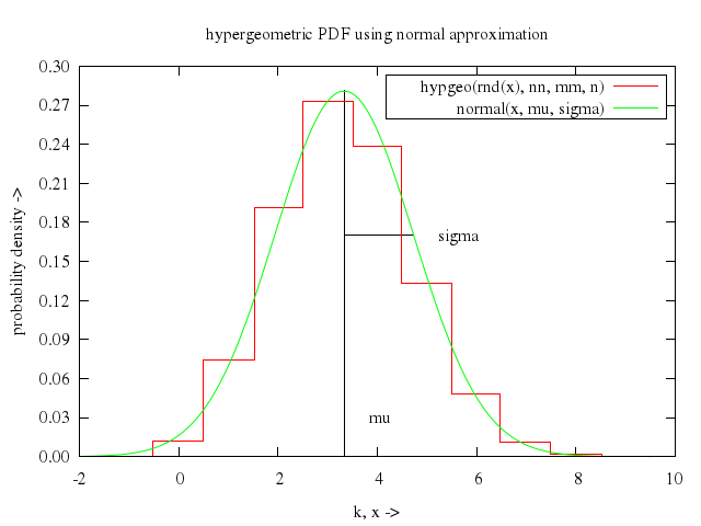
### 7
```ruby
# unset arrow
# unset label
#
# # Negative binomial PDF using gamma approximation
# r = 8; p = 0.6
# mu = r * (1.0 - p) / p
# sigma = sqrt(mu / p)
# lambda = p
# rho = r * (1.0 - p)
# xmin = floor(mu - r_sigma * sigma)
# xmin = xmin < r_xmin ? r_xmin : xmin
# xmax = ceil(mu + r_sigma * sigma)
# ymax = 1.1 * gmm((rho - 1) / lambda, rho, lambda) #mode of gamma PDF used
# set key box
# unset zeroaxis
# set xrange [xmin - 1 : xmax + 1]
# set yrange [0 : ymax]
# set xlabel "k, x ->"
# set ylabel "probability density ->"
# set ytics 0, ymax / 10.0, ymax
# set format x "%2.0f"
# set format y "%3.2f"
# set sample 200
# set title "negative binomial PDF using gamma approximation"
# set arrow from mu, 0 to mu, gmm(mu, rho, lambda) nohead
# set arrow from mu, gmm(mu + sigma, rho, lambda) \
# to mu + sigma, gmm(mu + sigma, rho, lambda) nohead
# set label "mu" at mu + 0.5, ymax / 10
# set label "sigma" at mu + 0.5 + sigma, gmm(mu + sigma, rho, lambda)
# plot negbin(rnd(x), r, p) with histeps, gmm(x, rho, lambda)
Numo.gnuplot do
unset :arrow
unset :label
run "r = 8; p = 0.6"
run "mu = r * (1.0 - p) / p"
run "sigma = sqrt(mu / p)"
run "lambda = p"
run "rho = r * (1.0 - p)"
run "xmin = floor(mu - r_sigma * sigma)"
run "xmin = xmin < r_xmin ? r_xmin : xmin"
run "xmax = ceil(mu + r_sigma * sigma)"
run "ymax = 1.1 * gmm((rho - 1) / lambda, rho, lambda) #mode of gamma PDF used"
set :key, :box
unset :zeroaxis
set xrange:"[xmin-1:xmax+1]"
set yrange:"[0:ymax]"
set xlabel:"k, x ->"
set ylabel:"probability density ->"
set ytics:'0,ymax/10.0,ymax'
set format_x:"%2.0f"
set format_y:"%3.2f"
set sample:200
set title:"negative binomial PDF using gamma approximation"
set :arrow, from:"mu, 0", to:"mu, gmm(mu, rho, lambda)", nohead:true
set :arrow, from:"mu, gmm(mu + sigma, rho, lambda)", to:"mu + sigma, gmm(mu + sigma, rho, lambda)", nohead:true
set label:"mu", at:"mu + 0.5, ymax / 10"
set label:"sigma", at:"mu + 0.5 + sigma, gmm(mu + sigma, rho, lambda)"
plot ["negbin(rnd(x), r, p)", with:"histeps"],
"gmm(x, rho, lambda)"
end
```
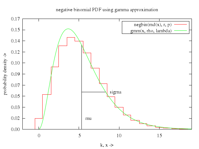
### 8
```ruby
# unset arrow
# unset label
#
# # Negative binomial PDF using normal approximation
# r = 8; p = 0.4
# mu = r * (1.0 - p) / p
# sigma = sqrt(mu / p)
# xmin = floor(mu - r_sigma * sigma)
# xmin = xmin < r_xmin ? r_xmin : xmin
# xmax = ceil(mu + r_sigma * sigma)
# ymax = 1.1 * negbin(floor((r-1)*(1-p)/p), r, p) #mode of gamma PDF used
# set key box
# unset zeroaxis
# set xrange [xmin - 1 : xmax + 1]
# set yrange [0 : ymax]
# set xlabel "k, x ->"
# set ylabel "probability density ->"
# set ytics 0, ymax / 10.0, ymax
# set format x "%2.0f"
# set format y "%3.2f"
# set sample 200
# set title "negative binomial PDF using normal approximation"
# set arrow from mu, 0 to mu, normal(mu, mu, sigma) nohead
# set arrow from mu, normal(mu + sigma, mu, sigma) \
# to mu + sigma, normal(mu + sigma, mu, sigma) nohead
# set label "mu" at mu + 0.5, ymax / 10
# set label "sigma" at mu + 0.5 + sigma, normal(mu + sigma, mu, sigma)
# plot negbin(rnd(x), r, p) with histeps, normal(x, mu, sigma)
Numo.gnuplot do
unset :arrow
unset :label
run "r = 8; p = 0.4"
run "mu = r * (1.0 - p) / p"
run "sigma = sqrt(mu / p)"
run "xmin = floor(mu - r_sigma * sigma)"
run "xmin = xmin < r_xmin ? r_xmin : xmin"
run "xmax = ceil(mu + r_sigma * sigma)"
run "ymax = 1.1 * negbin(floor((r-1)*(1-p)/p), r, p) #mode of gamma PDF used"
set :key, :box
unset :zeroaxis
set xrange:"[xmin-1:xmax+1]"
set yrange:"[0:ymax]"
set xlabel:"k, x ->"
set ylabel:"probability density ->"
set ytics:'0,ymax/10.0,ymax'
set format_x:"%2.0f"
set format_y:"%3.2f"
set sample:200
set title:"negative binomial PDF using normal approximation"
set :arrow, from:"mu, 0", to:"mu, normal(mu, mu, sigma)", nohead:true
set :arrow, from:"mu, normal(mu + sigma, mu, sigma)", to:"mu + sigma, normal(mu + sigma, mu, sigma)", nohead:true
set label:"mu", at:"mu + 0.5, ymax / 10"
set label:"sigma", at:"mu + 0.5 + sigma, normal(mu + sigma, mu, sigma)"
plot ["negbin(rnd(x), r, p)", with:"histeps"],
"normal(x, mu, sigma)"
end
```
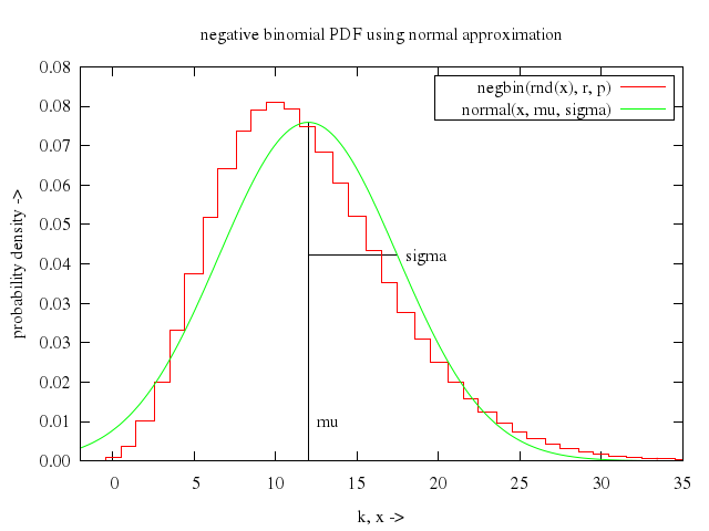
### 9
```ruby
# unset arrow
# unset label
#
# # Normal PDF using logistic approximation
# mu = 1.0; sigma = 1.5
# a = mu
# lambda = pi / (sqrt(3.0) * sigma)
# xmin = mu - r_sigma * sigma
# xmax = mu + r_sigma * sigma
# ymax = 1.1 * logistic(mu, a, lambda) #mode of logistic PDF used
# set key box
# unset zeroaxis
# set xrange [xmin: xmax]
# set yrange [0 : ymax]
# set xlabel "x ->"
# set ylabel "probability density ->"
# set ytics 0, ymax / 10.0, ymax
# set format x "%.1f"
# set format y "%.2f"
# set sample 200
# set title "normal PDF using logistic approximation"
# set arrow from mu,0 to mu, normal(mu, mu, sigma) nohead
# set arrow from mu, normal(mu + sigma, mu, sigma) \
# to mu + sigma, normal(mu + sigma, mu, sigma) nohead
# set label "mu" at mu + 0.5, ymax / 10
# set label "sigma" at mu + 0.5 + sigma, normal(mu + sigma, mu, sigma)
# plot logistic(x, a, lambda), normal(x, mu, sigma)
Numo.gnuplot do
unset :arrow
unset :label
run "mu = 1.0; sigma = 1.5"
run "a = mu"
run "lambda = pi / (sqrt(3.0) * sigma)"
run "xmin = mu - r_sigma * sigma"
run "xmax = mu + r_sigma * sigma"
run "ymax = 1.1 * logistic(mu, a, lambda) #mode of logistic PDF used"
set :key, :box
unset :zeroaxis
set xrange:"[xmin:xmax]"
set yrange:"[0:ymax]"
set xlabel:"x ->"
set ylabel:"probability density ->"
set ytics:'0,ymax/10.0,ymax'
set format_x:"%.1f"
set format_y:"%.2f"
set sample:200
set title:"normal PDF using logistic approximation"
set :arrow, from:"mu,0", to:"mu, normal(mu, mu, sigma)", nohead:true
set :arrow, from:"mu, normal(mu + sigma, mu, sigma)", to:"mu + sigma, normal(mu + sigma, mu, sigma)", nohead:true
set label:"mu", at:"mu + 0.5, ymax / 10"
set label:"sigma", at:"mu + 0.5 + sigma, normal(mu + sigma, mu, sigma)"
plot "logistic(x, a, lambda)",
"normal(x, mu, sigma)"
end
```
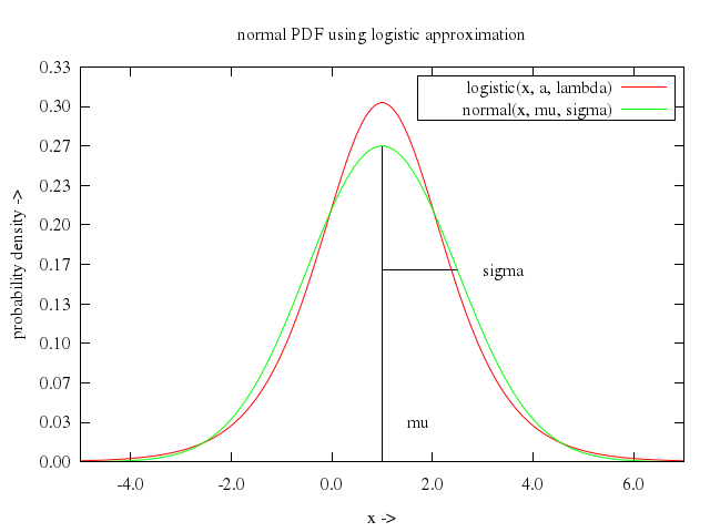
### 10
```ruby
# unset arrow
# unset label
#
# # Poisson PDF using normal approximation
# mu = 5.0
# sigma = sqrt(mu)
# xmin = floor(mu - r_sigma * sigma)
# xmin = xmin < r_xmin ? r_xmin : xmin
# xmax = ceil(mu + r_sigma * sigma)
# ymax = 1.1 * poisson(mu, mu) #mode of poisson PDF used
# set key box
# unset zeroaxis
# set xrange [xmin - 1 : xmax + 1]
# set yrange [0 : ymax]
# set xlabel "k, x ->"
# set ylabel "probability density ->"
# set ytics 0, ymax / 10.0, ymax
# set format x "%2.0f"
# set format y "%3.2f"
# set sample 200
# set title "poisson PDF using normal approximation"
# set arrow from mu, 0 to mu, normal(mu, mu, sigma) nohead
# set arrow from mu, normal(mu + sigma, mu, sigma) \
# to mu + sigma, normal(mu + sigma, mu, sigma) nohead
# set label "mu" at mu + 0.5, ymax / 10
# set label "sigma" at mu + 0.5 + sigma, normal(mu + sigma, mu, sigma)
# plot poisson(rnd(x), mu) with histeps, normal(x, mu, sigma)
Numo.gnuplot do
unset :arrow
unset :label
run "mu = 5.0"
run "sigma = sqrt(mu)"
run "xmin = floor(mu - r_sigma * sigma)"
run "xmin = xmin < r_xmin ? r_xmin : xmin"
run "xmax = ceil(mu + r_sigma * sigma)"
run "ymax = 1.1 * poisson(mu, mu) #mode of poisson PDF used"
set :key, :box
unset :zeroaxis
set xrange:"[xmin-1:xmax+1]"
set yrange:"[0:ymax]"
set xlabel:"k, x ->"
set ylabel:"probability density ->"
set ytics:'0,ymax/10.0,ymax'
set format_x:"%2.0f"
set format_y:"%3.2f"
set sample:200
set title:"poisson PDF using normal approximation"
set :arrow, from:"mu, 0", to:"mu, normal(mu, mu, sigma)", nohead:true
set :arrow, from:"mu, normal(mu + sigma, mu, sigma)", to:"mu + sigma, normal(mu + sigma, mu, sigma)", nohead:true
set label:"mu", at:"mu + 0.5, ymax / 10"
set label:"sigma", at:"mu + 0.5 + sigma, normal(mu + sigma, mu, sigma)"
plot ["poisson(rnd(x), mu)", with:"histeps"],
"normal(x, mu, sigma)"
end
```
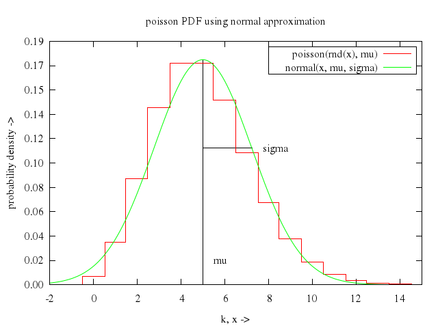
## probability (more)
[Original Demo](http://gnuplot.sourceforge.net/demo_4.6/prob.html)
### 1
```ruby
# # Demo Statistical Functions version 2.3
# #
# # Copyright (c) 1991, 1992 Jos van der Woude, [email protected]
#
# # History:
# # -- --- 1992 Jos van der Woude: 1st version
# # 06 Jun 2006 Dan Sebald: Added some variety and plotting techniques for
# # better visual effect. More tutorial in nature.
#
# print " Statistical Library Demo, version 2.3"
# print "\n Copyright (c) 1991, 1992, Jos van de Woude, [email protected]"
# print "\n\n\n\n\n\n\n"
# print "NOTE: contains 54 plots and consequently takes a lot of time to run"
# print " Press Ctrl-C to exit right now"
#
# load "stat.inc"
#
# eps = 1.0e-10 # Supposed to be float resolution (nice if were defined internally)
#
# ## Gamma function
# xmin = -5.5
# xmax = 5
# ymin = -10
# ymax = 10
# unset key
# set xzeroaxis
# gsampfunc(t,n) = t<0?0.5*1/(-t+1.0)**n:1.0-0.5*1/(t+1.0)**n
# set parametric
# set trange [-1:1]
# set sample 200
# set xrange [xmin : xmax]
# set yrange [ymin : ymax]
# set xlabel "x"
# set ylabel "gamma(x)"
# set arrow 1 from 0,ymin to 0,ymax nohead lt 0
# set arrow 2 from -1,ymin to -1,ymax nohead lt 0
# set arrow 3 from -2,ymin to -2,ymax nohead lt 0
# set arrow 4 from -3,ymin to -3,ymax nohead lt 0
# set arrow 5 from -4,ymin to -4,ymax nohead lt 0
# set arrow 6 from -5,ymin to -5,ymax nohead lt 0
# set title "gamma function, very useful function for probability"
# plot gsampfunc(5*t,5)-6, gamma(gsampfunc(5*t,5)-6) lt 1, \
# gsampfunc(5*t,5)-5, gamma(gsampfunc(5*t,5)-5) lt 1, \
# gsampfunc(5*t,4)-4, gamma(gsampfunc(5*t,4)-4) lt 1, \
# gsampfunc(5*t,3)-3, gamma(gsampfunc(5*t,3)-3) lt 1, \
# gsampfunc(5*t,2)-2, gamma(gsampfunc(5*t,2)-2) lt 1, \
# gsampfunc(5*t,1)-1, gamma(gsampfunc(5*t,1)-1) lt 1, \
# 5*gsampfunc(5*t,2), gamma(5*gsampfunc(5*t,2)) lt 1
Numo.gnuplot do
load "stat.inc"
run "eps = 1.0e-10 # Supposed to be float resolution (nice if were defined internally)"
run "xmin = -5.5"
run "xmax = 5"
run "ymin = -10"
run "ymax = 10"
unset :key
set :xzeroaxis
run "gsampfunc(t,n) = t<0?0.5*1/(-t+1.0)**n:1.0-0.5*1/(t+1.0)**n"
set :parametric
set trange:-1..1
set sample:200
set xrange:"[xmin:xmax]"
set yrange:"[ymin:ymax]"
set xlabel:"x"
set ylabel:"gamma(x)"
set :arrow, 1, from:'0,ymin', to:'0,ymax', nohead:true, lt:0
set :arrow, 2, from:"-1,ymin", to:"-1,ymax", nohead:true, lt:0
set :arrow, 3, from:"-2,ymin", to:"-2,ymax", nohead:true, lt:0
set :arrow, 4, from:"-3,ymin", to:"-3,ymax", nohead:true, lt:0
set :arrow, 5, from:"-4,ymin", to:"-4,ymax", nohead:true, lt:0
set :arrow, 6, from:"-5,ymin", to:"-5,ymax", nohead:true, lt:0
set title:"gamma function, very useful function for probability"
plot "gsampfunc(5*t,5)-6",
["gamma(gsampfunc(5*t,5)-6)", lt:1],
"gsampfunc(5*t,5)-5",
["gamma(gsampfunc(5*t,5)-5)", lt:1],
"gsampfunc(5*t,4)-4",
["gamma(gsampfunc(5*t,4)-4)", lt:1],
"gsampfunc(5*t,3)-3",
["gamma(gsampfunc(5*t,3)-3)", lt:1],
"gsampfunc(5*t,2)-2",
["gamma(gsampfunc(5*t,2)-2)", lt:1],
"gsampfunc(5*t,1)-1",
["gamma(gsampfunc(5*t,1)-1)", lt:1],
"5*gsampfunc(5*t,2)",
["gamma(5*gsampfunc(5*t,2))", lt:1]
end
```
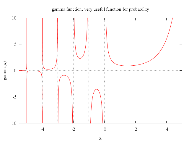
### 2
```ruby
# ymin = ymin/2
# ymax = ymax/2
# set yrange [ymin:ymax]
# set ylabel "lgamma(x)"
# set arrow 1 from 0,ymin to 0,ymax nohead lt 0
# set arrow 2 from -1,ymin to -1,ymax nohead lt 0
# set arrow 3 from -2,ymin to -2,ymax nohead lt 0
# set arrow 4 from -3,ymin to -3,ymax nohead lt 0
# set arrow 5 from -4,ymin to -4,ymax nohead lt 0
# set arrow 6 from -5,ymin to -5,ymax nohead lt 0
# set title "log gamma function, similarly very useful function"
# plot gsampfunc(5*t,5)-6, lgamma(gsampfunc(5*t,5)-6) lt 1, \
# gsampfunc(5*t,5)-5, lgamma(gsampfunc(5*t,5)-5) lt 1, \
# gsampfunc(5*t,4)-4, lgamma(gsampfunc(5*t,4)-4) lt 1, \
# gsampfunc(5*t,3)-3, lgamma(gsampfunc(5*t,3)-3) lt 1, \
# gsampfunc(5*t,3)-2, lgamma(gsampfunc(5*t,3)-2) lt 1, \
# gsampfunc(5*t,3)-1, lgamma(gsampfunc(5*t,3)-1) lt 1, \
# 5*gsampfunc(5*t,3), lgamma(5*gsampfunc(5*t,3)) lt 1
Numo.gnuplot do
run "ymin = ymin/2"
run "ymax = ymax/2"
set yrange:"[ymin:ymax]"
set ylabel:"lgamma(x)"
set :arrow, 1, from:'0,ymin', to:'0,ymax', nohead:true, lt:0
set :arrow, 2, from:"-1,ymin", to:"-1,ymax", nohead:true, lt:0
set :arrow, 3, from:"-2,ymin", to:"-2,ymax", nohead:true, lt:0
set :arrow, 4, from:"-3,ymin", to:"-3,ymax", nohead:true, lt:0
set :arrow, 5, from:"-4,ymin", to:"-4,ymax", nohead:true, lt:0
set :arrow, 6, from:"-5,ymin", to:"-5,ymax", nohead:true, lt:0
set title:"log gamma function, similarly very useful function"
plot "gsampfunc(5*t,5)-6",
["lgamma(gsampfunc(5*t,5)-6)", lt:1],
"gsampfunc(5*t,5)-5",
["lgamma(gsampfunc(5*t,5)-5)", lt:1],
"gsampfunc(5*t,4)-4",
["lgamma(gsampfunc(5*t,4)-4)", lt:1],
"gsampfunc(5*t,3)-3",
["lgamma(gsampfunc(5*t,3)-3)", lt:1],
"gsampfunc(5*t,3)-2",
["lgamma(gsampfunc(5*t,3)-2)", lt:1],
"gsampfunc(5*t,3)-1",
["lgamma(gsampfunc(5*t,3)-1)", lt:1],
"5*gsampfunc(5*t,3)",
["lgamma(5*gsampfunc(5*t,3))", lt:1]
end
```
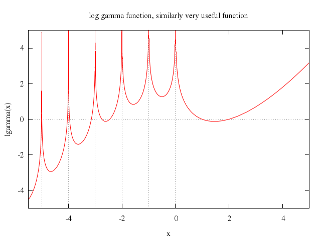
### 3
```ruby
# reset
#
# # Arcsinus PDF and CDF
# r = 2.0
# mu = 0.0
# sigma = r / sqrt2
# xmin = -(r+1)
# xmax = r+1
# unset key
# set zeroaxis
# set xrange [xmin : xmax]
# set yrange [-0.2 : 1.2]
# set xlabel "x ->"
# set ylabel "probability density ->"
# set xtics autofreq
# set ytics autofreq
# set format x "%.1f"
# set format y "%.1f"
# set sample 50*xmax+1
# set title "arcsin PDF with r = 2.0"
# plot arcsin(x, r)
Numo.gnuplot do
reset
run "r = 2.0"
run "mu = 0.0"
run "sigma = r / sqrt2"
run "xmin = -(r+1)"
run "xmax = r+1"
unset :key
set :zeroaxis
set xrange:"[xmin:xmax]"
set yrange:-0.2..1.2
set xlabel:"x ->"
set ylabel:"probability density ->"
set xtics:"autofreq"
set ytics:"autofreq"
set format_x:"%.1f"
set format_y:"%.1f"
set sample:'50*xmax+1'
set title:"arcsin PDF with r = 2.0"
plot "arcsin(x, r)"
end
```
### 4
```ruby
# set title "arcsin CDF with r = 2.0"
# set yrange [-0.2 : 1.2]
# plot carcsin(x, r)
Numo.gnuplot do
set title:"arcsin CDF with r = 2.0"
set yrange:-0.2..1.2
plot "carcsin(x, r)"
end
```
### 5
```ruby
# # Beta PDF and CDF
# p = 5.0; q = 3.0
# mu = p / (p + q)
# sigma = sqrt(p**q) / ((p + q ) * sqrt(p + q + 1.0))
# xmin = 0.0
# xmax = 1.0
# #Mode of beta PDF used
# ymax = (p < 1.0 || q < 1.0) ? 2.0 : 1.4 * beta((p - 1.0)/(p + q - 2.0), p, q)
# set key right box
# set zeroaxis
# set xrange [xmin : xmax]
# set yrange [0 : ymax]
# set xlabel "x ->"
# set ylabel "probability density ->"
# set xtics autofreq
# set ytics autofreq
# set format x "%.1f"
# set format y "%.1f"
# set sample 200
# set title "beta PDF"
# plot beta(x, 0.5, 0.7) title "p = 0.5, q = 0.7", \
# beta(x, 5.0, 3.0) title "p = 5.0, q = 3.0", \
# beta(x, 0.5, 2.5) title "p = 0.5, q = 2.5"
Numo.gnuplot do
run "p = 5.0; q = 3.0"
run "mu = p / (p + q)"
run "sigma = sqrt(p**q) / ((p + q ) * sqrt(p + q + 1.0))"
run "xmin = 0.0"
run "xmax = 1.0"
run "ymax = (p < 1.0 || q < 1.0) ? 2.0 : 1.4 * beta((p - 1.0)/(p + q - 2.0), p, q)"
set :key, :right, :box
set :zeroaxis
set xrange:"[xmin:xmax]"
set yrange:"[0:ymax]"
set xlabel:"x ->"
set ylabel:"probability density ->"
set xtics:"autofreq"
set ytics:"autofreq"
set format_x:"%.1f"
set format_y:"%.1f"
set sample:200
set title:"beta PDF"
plot ["beta(x, 0.5, 0.7)", title:"p = 0.5, q = 0.7"],
["beta(x, 5.0, 3.0)", title:"p = 5.0, q = 3.0"],
["beta(x, 0.5, 2.5)", title:"p = 0.5, q = 2.5"]
end
```
### 6
```ruby
# set yrange [0:1.1]
# set title "incomplete beta CDF"
# set key left box
# plot cbeta(x, 0.5, 0.7) title "p = 0.5, q = 0.7", \
# cbeta(x, 5.0, 3.0) title "p = 5.0, q = 3.0", \
# cbeta(x, 0.5, 2.5) title "p = 0.5, q = 2.5"
Numo.gnuplot do
set yrange:0..1.1
set title:"incomplete beta CDF"
set :key, :left, :box
plot ["cbeta(x, 0.5, 0.7)", title:"p = 0.5, q = 0.7"],
["cbeta(x, 5.0, 3.0)", title:"p = 5.0, q = 3.0"],
["cbeta(x, 0.5, 2.5)", title:"p = 0.5, q = 2.5"]
end
```
### 7
```ruby
# # Binomial PDF and CDF
# n = 25; p = 0.15
# mu = n * p
# sigma = sqrt(n * p * (1.0 - p))
# xmin = int(mu - 4.0 * sigma)
# xmin = xmin < -2 ? -2 : xmin
# xmax = int(mu + 4.0 * sigma)
# xmax = xmax < n+2 ? n+2 : xmax
# ymax = 1.1 * binom(int((n+1)*p), n, p) #Mode of binomial PDF used
# unset key
# unset zeroaxis
# set xrange [xmin : xmax]
# set yrange [0 : ymax]
# set xlabel "k ->"
# set ylabel "probability density ->"
# set ytics 0, ymax / 10, ymax
# set format x "%2.0f"
# set format y "%3.2f"
# set sample (xmax - xmin) + 1
# set title "binomial PDF with n = 25, p = 0.15"
# plot binom(x, n, p) with impulses
Numo.gnuplot do
run "n = 25; p = 0.15"
run "mu = n * p"
run "sigma = sqrt(n * p * (1.0 - p))"
run "xmin = int(mu - 4.0 * sigma)"
run "xmin = xmin < -2 ? -2 : xmin"
run "xmax = int(mu + 4.0 * sigma)"
run "xmax = xmax < n+2 ? n+2 : xmax"
run "ymax = 1.1 * binom(int((n+1)*p), n, p) #Mode of binomial PDF used"
unset :key
unset :zeroaxis
set xrange:"[xmin:xmax]"
set yrange:"[0:ymax]"
set xlabel:"k ->"
set ylabel:"probability density ->"
set ytics:'0,ymax/10,ymax'
set format_x:"%2.0f"
set format_y:"%3.2f"
set sample:'(xmax - xmin)+1'
set title:"binomial PDF with n = 25, p = 0.15"
plot "binom(x, n, p)", with:"impulses"
end
```
### 8
```ruby
# set ytics autofreq
# set xzeroaxis
# set title "binomial CDF with n = 25, p = 0.15"
# set yrange [-0.1 : 1.1]
# set ytics 0, 0.1, 1.0
# plot cbinom(x, n, p) with steps
Numo.gnuplot do
set ytics:"autofreq"
set :xzeroaxis
set title:"binomial CDF with n = 25, p = 0.15"
set yrange:-0.1..1.1
set ytics:[0,0.1,1.0]
plot "cbinom(x, n, p)", with:"steps"
end
```
### 9
```ruby
# # Cauchy PDF and CDF
# a = 0.0; b = 2.0
# #cauchy PDF has no moments
# xmin = a - 5.0 * b
# xmax = a + 5.0 * b
# ymax = 1.1 * cauchy(a, a, b) #Mode of cauchy PDF used
# set key left box
# set zeroaxis
# set xlabel "x ->"
# set ylabel "probability density ->"
# set xtics autofreq
# set ytics autofreq
# set format x "%.1f"
# set format y "%.2f"
# set sample 100
# set title "cauchy PDF"
# a=0
# b=2
# plot [xmin:xmax] [0:ymax] cauchy(x, 0, 2) title "a = 0, b = 2", \
# cauchy(x, 0, 4) title "a = 0, b = 4"
Numo.gnuplot do
run "a = 0.0; b = 2.0"
run "xmin = a - 5.0 * b"
run "xmax = a + 5.0 * b"
run "ymax = 1.1 * cauchy(a, a, b) #Mode of cauchy PDF used"
set :key, :left, :box
set :zeroaxis
set xlabel:"x ->"
set ylabel:"probability density ->"
set xtics:"autofreq"
set ytics:"autofreq"
set format_x:"%.1f"
set format_y:"%.2f"
set sample:100
set title:"cauchy PDF"
run "a=0"
run "b=2"
plot "[xmin:xmax]","[0:ymax]",
["cauchy(x, 0, 2)", title:"a = 0, b = 2"],
["cauchy(x, 0, 4)", title:"a = 0, b = 4"]
end
```
### 10
```ruby
# set title "cauchy CDF"
# plot [xmin:xmax] [0:1.0] ccauchy(x, 0, 2) title "a = 0, b = 2", \
# ccauchy(x, 0, 4) title "a = 0, b = 4"
Numo.gnuplot do
set title:"cauchy CDF"
plot "[xmin:xmax]", 0..1.0,
["ccauchy(x, 0, 2)", title:"a = 0, b = 2"],
["ccauchy(x, 0, 4)", title:"a = 0, b = 4"]
end
```
### 11
```ruby
# # Chi-square PDF and CDF
# k = 4.0
# mu = k
# sigma = sqrt(2.0 * k)
# xmin = mu - 4.0 * sigma
# xmin = xmin < 0 ? 0 : xmin
# xmax = int(mu + 4.0 * sigma)
# k = 2.0
# ymax = (k > 2.0 ? 1.1*chisq(k - 2.0, k) : 0.5) #Mode of chi PDF used
# set key right box
# set zeroaxis
# set xrange [xmin+eps : xmax] #Discontinuity at zero for k < 2
# set yrange [0:ymax]
# set xlabel "x ->"
# set ylabel "probability density ->"
# set xtics autofreq
# set ytics autofreq
# set format x "%.1f"
# set format y "%.2f"
# set sample 100
# set title "chi-square PDF"
# set key right box
# set samples 15*20+1
# keystr(k) = sprintf("k = %d", k)
# plot k = 1, x==0?1/0:chisq(x, k) title keystr(k), \
# k = 2, x==0?1/0:chisq(x, k) title keystr(k), \
# k = 3, chisq(x, k) title keystr(k), \
# k = 4, chisq(x, k) title keystr(k), \
# k = 5, chisq(x, k) title keystr(k), \
# k = 6, chisq(x, k) title keystr(k), \
# k = 7, chisq(x, k) title keystr(k), \
# k = 8, chisq(x, k) title keystr(k)
Numo.gnuplot do
run "k = 4.0"
run "mu = k"
run "sigma = sqrt(2.0 * k)"
run "xmin = mu - 4.0 * sigma"
run "xmin = xmin < 0 ? 0 : xmin"
run "xmax = int(mu + 4.0 * sigma)"
run "k = 2.0"
run "ymax = (k > 2.0 ? 1.1*chisq(k - 2.0, k) : 0.5) #Mode of chi PDF used"
set :key, :right, :box
set :zeroaxis
set xrange:"[xmin+eps:xmax]" #Discontinuity at "zero" for k < 2
set yrange:"[0:ymax]"
set xlabel:"x ->"
set ylabel:"probability density ->"
set xtics:"autofreq"
set ytics:"autofreq"
set format_x:"%.1f"
set format_y:"%.2f"
set sample:100
set title:"chi-square PDF"
set :key, :right, :box
set samples:'15*20+1'
run "keystr(k) = sprintf(\"k = %d\", k)"
plot "k=1",
["x==0?1/0:chisq(x, k)", title_nq:'keystr(k)'],
"k=2",
["x==0?1/0:chisq(x, k)", title_nq:'keystr(k)'],
"k=3",
["chisq(x, k)", title_nq:'keystr(k)'],
"k=4",
["chisq(x, k)", title_nq:'keystr(k)'],
"k=5",
["chisq(x, k)", title_nq:'keystr(k)'],
"k=6",
["chisq(x, k)", title_nq:'keystr(k)'],
"k=7",
["chisq(x, k)", title_nq:'keystr(k)'],
"k=8",
["chisq(x, k)", title_nq:'keystr(k)']
end
```
### 12
```ruby
# set yrange [0:1.1]
# set key bottom right box
# set title "chi-square CDF"
# plot k = 1, cchisq(x, k) title keystr(k), \
# k = 2, cchisq(x, k) title keystr(k), \
# k = 3, cchisq(x, k) title keystr(k), \
# k = 4, cchisq(x, k) title keystr(k), \
# k = 5, cchisq(x, k) title keystr(k), \
# k = 6, cchisq(x, k) title keystr(k), \
# k = 7, cchisq(x, k) title keystr(k), \
# k = 8, cchisq(x, k) title keystr(k)
Numo.gnuplot do
set yrange:0..1.1
set :key, :bottom, :right, :box
set title:"chi-square CDF"
plot "k=1",
["cchisq(x, k)", title_nq:'keystr(k)'],
"k=2",
["cchisq(x, k)", title_nq:'keystr(k)'],
"k=3",
["cchisq(x, k)", title_nq:'keystr(k)'],
"k=4",
["cchisq(x, k)", title_nq:'keystr(k)'],
"k=5",
["cchisq(x, k)", title_nq:'keystr(k)'],
"k=6",
["cchisq(x, k)", title_nq:'keystr(k)'],
"k=7",
["cchisq(x, k)", title_nq:'keystr(k)'],
"k=8",
["cchisq(x, k)", title_nq:'keystr(k)']
end
```
### 13
```ruby
# # Erlang PDF and CDF
# lambda = 1.0; n = 2.0
# mu = n / lambda
# sigma = sqrt(n) / lambda
# xmax = int(mu + 5.0 * sigma)
# n = 1.0
# ymax = n < 2.0 ? 1.0 : 1.1 * erlang((n - 1.0) / lambda, n, lambda) #Mode of erlang PDF used
# set zeroaxis
# set xlabel "x ->"
# set ylabel "probability density ->"
# set xtics autofreq
# set ytics autofreq
# set format x "%.1f"
# set format y "%.1f"
# set sample 100
# set title "erlang PDF"
# set key top right box
# l1 = 1.0; l2 = 0.5
# set arrow 1 from 2,0.8 to 0.33,erlang(0.33,1,l1)
# set arrow 2 from 2,0.8 to 0.33,erlang(0.33,1,l2)
# set label 1 "n = 1, exponential r.v." at 2.1,0.8 left
# keystr(n,lambda) = sprintf("lambda = %0.1f, n = %d", lambda, n)
# plot [0:xmax] [0:ymax] n = 1, lambda = l1, erlang(x, n, lambda) title keystr(n,lambda), \
# n = 1, lambda = l2, erlang(x, n, lambda) title keystr(n,lambda), \
# n = 2, lambda = l1, erlang(x, n, lambda) title keystr(n,lambda), \
# n = 2, lambda = l2, erlang(x, n, lambda) title keystr(n,lambda)
Numo.gnuplot do
run "lambda = 1.0; n = 2.0"
run "mu = n / lambda"
run "sigma = sqrt(n) / lambda"
run "xmax = int(mu + 5.0 * sigma)"
run "n = 1.0"
run "ymax = n < 2.0 ? 1.0 : 1.1 * erlang((n - 1.0) / lambda, n, lambda) #Mode of erlang PDF used"
set :zeroaxis
set xlabel:"x ->"
set ylabel:"probability density ->"
set xtics:"autofreq"
set ytics:"autofreq"
set format_x:"%.1f"
set format_y:"%.1f"
set sample:100
set title:"erlang PDF"
set :key, :top, :right, :box
run "l1 = 1.0; l2 = 0.5"
set :arrow, 1, from:[2,0.8], to:"0.33,erlang(0.33,1,l1)"
set :arrow, 2, from:[2,0.8], to:"0.33,erlang(0.33,1,l2)"
set :label, 1, "n = 1, exponential r.v.", at:[2.1,0.8], left:true
run "keystr(n,lambda) = sprintf(\"lambda = %0.1f, n = %d\", lambda, n)"
plot "[0:xmax]","[0:ymax]",
"n=1",
"lambda=l1",
["erlang(x, n, lambda)", title_nq:'keystr(n,lambda)'],
"n=1",
"lambda=l2",
["erlang(x, n, lambda)", title_nq:'keystr(n,lambda)'],
"n=2",
"lambda=l1",
["erlang(x, n, lambda)", title_nq:'keystr(n,lambda)'],
"n=2",
"lambda=l2",
["erlang(x, n, lambda)", title_nq:'keystr(n,lambda)']
end
```
### 14
```ruby
# unset label 1
# unset arrow 1; unset arrow 2
# set title "erlang CDF"
# set key bottom right box
# plot [0:xmax] [0:1.1] n = 1, lambda = l1, cerlang(x, n, lambda) title keystr(n,lambda), \
# n = 1, lambda = l2, cerlang(x, n, lambda) title keystr(n,lambda), \
# n = 2, lambda = l1, cerlang(x, n, lambda) title keystr(n,lambda), \
# n = 2, lambda = l2, cerlang(x, n, lambda) title keystr(n,lambda)
Numo.gnuplot do
unset label:1
unset :arrow, 1; unset :arrow, 2
set title:"erlang CDF"
set :key, :bottom, :right, :box
plot "[0:xmax]", 0..1.1,
"n=1",
"lambda=l1",
["cerlang(x, n, lambda)", title_nq:'keystr(n,lambda)'],
"n=1",
"lambda=l2",
["cerlang(x, n, lambda)", title_nq:'keystr(n,lambda)'],
"n=2",
"lambda=l1",
["cerlang(x, n, lambda)", title_nq:'keystr(n,lambda)'],
"n=2",
"lambda=l2",
["cerlang(x, n, lambda)", title_nq:'keystr(n,lambda)']
end
```
### 15
```ruby
# # Thanks to [email protected] for telling us about this.
# # Extreme (Gumbel extreme value) PDF and CDF
# alpha = 1.0; u = 0.0
# mu = u + (0.577215665/alpha) # Euler's constant
# sigma = pi/(sqrt(6.0)*alpha)
# xmin = mu - 6.0 * sigma
# xmax = mu + 6.0 * sigma
# ymax = 1.1 * extreme(u, u, alpha) #Mode of extreme PDF used
# ymax = int(10*ymax)/10.0
# set zeroaxis
# set xlabel "x ->"
# set ylabel "probability density ->"
# set xtics autofreq
# set ytics autofreq
# set format x "%.1f"
# set format y "%.2f"
# set sample 100
# set title "extreme PDF"
# set key top left box
# plot [xmin:xmax] [0:ymax] extreme(x, 1.0, 0.5) title "alpha = 0.5, u = 1.0", \
# extreme(x, 0.0, 1.0) title "alpha = 1.0, u = 0.0"
Numo.gnuplot do
run "alpha = 1.0; u = 0.0"
run "mu = u + (0.577215665/alpha) # Euler's constant"
run "sigma = pi/(sqrt(6.0)*alpha)"
run "xmin = mu - 6.0 * sigma"
run "xmax = mu + 6.0 * sigma"
run "ymax = 1.1 * extreme(u, u, alpha) #Mode of extreme PDF used"
run "ymax = int(10*ymax)/10.0"
set :zeroaxis
set xlabel:"x ->"
set ylabel:"probability density ->"
set xtics:"autofreq"
set ytics:"autofreq"
set format_x:"%.1f"
set format_y:"%.2f"
set sample:100
set title:"extreme PDF"
set :key, :top, :left, :box
plot "[xmin:xmax]","[0:ymax]",
["extreme(x, 1.0, 0.5)", title:"alpha = 0.5, u = 1.0"],
["extreme(x, 0.0, 1.0)", title:"alpha = 1.0, u = 0.0"]
end
```
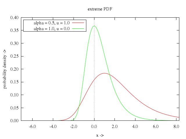
### 16
```ruby
# set title "extreme CDF"
# plot [xmin:xmax] [0:1.1] cextreme(x, 1.0, 0.5) title "alpha = 0.5, u = 1.0", \
# cextreme(x, 0.0, 1.0) title "alpha = 1.0, u = 0.0"
Numo.gnuplot do
set title:"extreme CDF"
plot "[xmin:xmax]", 0..1.1,
["cextreme(x, 1.0, 0.5)", title:"alpha = 0.5, u = 1.0"],
["cextreme(x, 0.0, 1.0)", title:"alpha = 1.0, u = 0.0"]
end
```
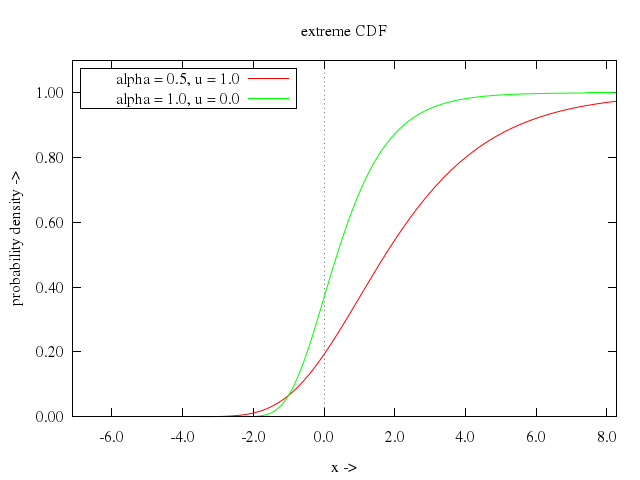
### 17
```ruby
# # F PDF and CDF
# df1 = 5.0; df2 = 9.0
# mu = df2 < 2.0 ? 1.0 : df2 / (df2 - 2.0)
# sigma = df2 < 4.0 ? 1.0 : mu * sqrt(2.0 * (df1 + df2 - 2.0) / (df1 * (df2 - 4.0)))
# xmin = mu - 3.0 * sigma
# xmin = xmin < 0 ? 0 : xmin
# xmax = int(mu + 3.0 * sigma)
# #Mode of F PDF used
# ymax = df1 < 3.0 ? 1.0 : 1.1 * f((df1 / 2.0 - 1.0) / (df1 / 2.0 + df1 / df2), df1, df2)
# set zeroaxis
# set xlabel "x ->"
# set ylabel "probability density ->"
# set xtics autofreq
# set ytics autofreq
# set format x "%.1f"
# set format y "%.2f"
# set sample 100
# set title "F PDF"
# set key right box
# plot [xmin:xmax] [0:ymax] f(x, 5.0, 9.0) title "df1 = 5, df2 = 9", \
# f(x, 7.0, 6.0) title "df1 = 7, df2 = 6"
Numo.gnuplot do
run "df1 = 5.0; df2 = 9.0"
run "mu = df2 < 2.0 ? 1.0 : df2 / (df2 - 2.0)"
run "sigma = df2 < 4.0 ? 1.0 : mu * sqrt(2.0 * (df1 + df2 - 2.0) / (df1 * (df2 - 4.0)))"
run "xmin = mu - 3.0 * sigma"
run "xmin = xmin < 0 ? 0 : xmin"
run "xmax = int(mu + 3.0 * sigma)"
run "ymax = df1 < 3.0 ? 1.0 : 1.1 * f((df1 / 2.0 - 1.0) / (df1 / 2.0 + df1 / df2), df1, df2)"
set :zeroaxis
set xlabel:"x ->"
set ylabel:"probability density ->"
set xtics:"autofreq"
set ytics:"autofreq"
set format_x:"%.1f"
set format_y:"%.2f"
set sample:100
set title:"F PDF"
set :key, :right, :box
plot "[xmin:xmax]","[0:ymax]",
["f(x, 5.0, 9.0)", title:"df1 = 5, df2 = 9"],
["f(x, 7.0, 6.0)", title:"df1 = 7, df2 = 6"]
end
```
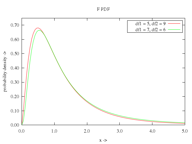
### 18
```ruby
# set title "F CDF"
# set key left box
# plot [xmin:xmax] [0:1.1] cf(x, 5.0, 9.0) title "df1 = 5, df2 = 9", \
# cf(x, 7.0, 6.0) title "df1 = 7, df2 = 6"
Numo.gnuplot do
set title:"F CDF"
set :key, :left, :box
plot "[xmin:xmax]", 0..1.1,
["cf(x, 5.0, 9.0)", title:"df1 = 5, df2 = 9"],
["cf(x, 7.0, 6.0)", title:"df1 = 7, df2 = 6"]
end
```
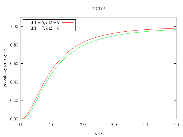
### 19
```ruby
# # Gamma PDF and incomplete gamma CDF
# rho = 1.0; lambda = 1.3
# mu = rho / lambda
# sigma = sqrt(rho) / lambda
# xmin = mu - 4.0 * sigma
# xmin = xmin < 0 ? 0 : xmin
# xmax = mu + 4.0 * sigma
# ymax = rho < 1.0 ? 2.0 : 1.1 * gmm((rho - 1.0) / lambda, rho, lambda) #Mode of gamma pdf used
# set zeroaxis
# set xlabel "x ->"
# set ylabel "probability density ->"
# set xtics autofreq
# set ytics autofreq
# set format x "%.1f"
# set format y "%.1f"
# set sample 100
# set title "gamma PDF"
# set key right
# r1 = 0.5; r2 = 1.0; r3 = 1.0; r4 = 1.3; r5 = 2.0; r6 = 4.0; r7 = 6.0
# l1 = 1.0; l2 = 1.0; l3 = 1.3; l4 = 1.3; l5 = 2.0; l6 = 2.0; l7 = 2.0
# set arrow 1 from 1,1.3 to 0.15,gmm(0.15,r1,l1)
# set label 1 "rho < 1, tends to infinity" at 1.1,1.3 left
# set arrow 2 from 1.15,1.1 to 0.35,gmm(0.35,r3,l3)
# set label 2 "rho = 1, finite, nonzero limit" at 1.25,1.1 left
# set arrow 3 from 1.5,0.9 to 1.0,gmm(1.0,r5,l5)
# set label 3 "rho > 1, tends to zero" at 1.6,0.9 left
# keystr(rho,lambda) = sprintf("rho = %0.1f, lambda = %0.1f", rho, lambda)
# plot [0:5] [0:1.5] rho = r1, lambda = l1, gmm(x, rho, lambda) title keystr(rho,lambda), \
# rho = r2, lambda = l2, gmm(x, rho, lambda) title keystr(rho,lambda), \
# rho = r3, lambda = l3, gmm(x, rho, lambda) title keystr(rho,lambda), \
# rho = r4, lambda = l4, gmm(x, rho, lambda) title keystr(rho,lambda), \
# rho = r5, lambda = l5, gmm(x, rho, lambda) title keystr(rho,lambda), \
# rho = r6, lambda = l6, gmm(x, rho, lambda) title keystr(rho,lambda), \
# rho = r7, lambda = l7, gmm(x, rho, lambda) title keystr(rho,lambda)
Numo.gnuplot do
run "rho = 1.0; lambda = 1.3"
run "mu = rho / lambda"
run "sigma = sqrt(rho) / lambda"
run "xmin = mu - 4.0 * sigma"
run "xmin = xmin < 0 ? 0 : xmin"
run "xmax = mu + 4.0 * sigma"
run "ymax = rho < 1.0 ? 2.0 : 1.1 * gmm((rho - 1.0) / lambda, rho, lambda) #Mode of gamma pdf used"
set :zeroaxis
set xlabel:"x ->"
set ylabel:"probability density ->"
set xtics:"autofreq"
set ytics:"autofreq"
set format_x:"%.1f"
set format_y:"%.1f"
set sample:100
set title:"gamma PDF"
set :key, :right
run "r1 = 0.5; r2 = 1.0; r3 = 1.0; r4 = 1.3; r5 = 2.0; r6 = 4.0; r7 = 6.0"
run "l1 = 1.0; l2 = 1.0; l3 = 1.3; l4 = 1.3; l5 = 2.0; l6 = 2.0; l7 = 2.0"
set :arrow, 1, from:[1,1.3], to:"0.15,gmm(0.15,r1,l1)"
set :label, 1, "rho < 1, tends to infinity", at:[1.1,1.3], left:true
set :arrow, 2, from:[1.15,1.1], to:"0.35,gmm(0.35,r3,l3)"
set :label, 2, "rho = 1, finite, nonzero limit", at:[1.25,1.1], left:true
set :arrow, 3, from:[1.5,0.9], to:"1.0,gmm(1.0,r5,l5)"
set :label, 3, "rho > 1, tends to zero", at:[1.6,0.9], left:true
run "keystr(rho,lambda) = sprintf(\"rho = %0.1f, lambda = %0.1f\", rho, lambda)"
plot 0..5, 0..1.5,
"rho=r1",
"lambda=l1",
["gmm(x, rho, lambda)", title_nq:'keystr(rho,lambda)'],
"rho=r2",
"lambda=l2",
["gmm(x, rho, lambda)", title_nq:'keystr(rho,lambda)'],
"rho=r3",
"lambda=l3",
["gmm(x, rho, lambda)", title_nq:'keystr(rho,lambda)'],
"rho=r4",
"lambda=l4",
["gmm(x, rho, lambda)", title_nq:'keystr(rho,lambda)'],
"rho=r5",
"lambda=l5",
["gmm(x, rho, lambda)", title_nq:'keystr(rho,lambda)'],
"rho=r6",
"lambda=l6",
["gmm(x, rho, lambda)", title_nq:'keystr(rho,lambda)'],
"rho=r7",
"lambda=l7",
["gmm(x, rho, lambda)", title_nq:'keystr(rho,lambda)']
end
```
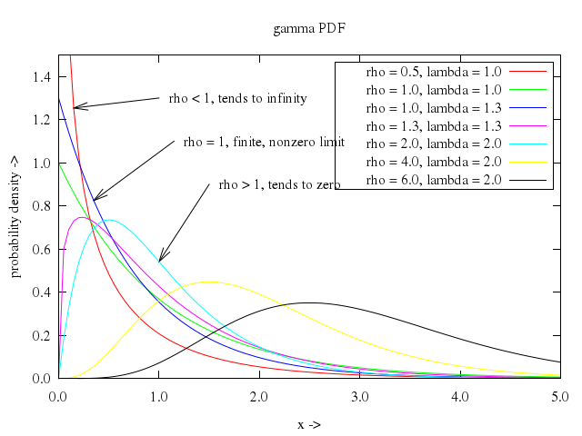
### 20
```ruby
# unset label 1; unset label 2; unset label 3
# unset arrow 1; unset arrow 2; unset arrow 3
# set title "incomplete gamma CDF"
# set key right bottom
# plot [0:5] [0:1.1] rho = r1, lambda = l1, cgmm(x, rho, lambda) title keystr(rho,lambda), \
# rho = r2, lambda = l2, cgmm(x, rho, lambda) title keystr(rho,lambda), \
# rho = r3, lambda = l3, cgmm(x, rho, lambda) title keystr(rho,lambda), \
# rho = r4, lambda = l4, cgmm(x, rho, lambda) title keystr(rho,lambda), \
# rho = r5, lambda = l5, cgmm(x, rho, lambda) title keystr(rho,lambda), \
# rho = r6, lambda = l6, cgmm(x, rho, lambda) title keystr(rho,lambda), \
# rho = r7, lambda = l7, cgmm(x, rho, lambda) title keystr(rho,lambda)
Numo.gnuplot do
unset label:1; unset label:2; unset label:3
unset :arrow, 1; unset :arrow, 2; unset :arrow, 3
set title:"incomplete gamma CDF"
set :key, :right, :bottom
plot 0..5, 0..1.1,
"rho=r1",
"lambda=l1",
["cgmm(x, rho, lambda)", title_nq:'keystr(rho,lambda)'],
"rho=r2",
"lambda=l2",
["cgmm(x, rho, lambda)", title_nq:'keystr(rho,lambda)'],
"rho=r3",
"lambda=l3",
["cgmm(x, rho, lambda)", title_nq:'keystr(rho,lambda)'],
"rho=r4",
"lambda=l4",
["cgmm(x, rho, lambda)", title_nq:'keystr(rho,lambda)'],
"rho=r5",
"lambda=l5",
["cgmm(x, rho, lambda)", title_nq:'keystr(rho,lambda)'],
"rho=r6",
"lambda=l6",
["cgmm(x, rho, lambda)", title_nq:'keystr(rho,lambda)'],
"rho=r7",
"lambda=l7",
["cgmm(x, rho, lambda)", title_nq:'keystr(rho,lambda)']
end
```
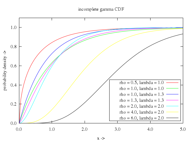
### 21
```ruby
# # Geometric PDF and CDF
# p = 0.4
# mu = (1.0 - p) / p
# sigma = sqrt(mu / p)
# xmin = int(mu - 4.0 * sigma)
# xmin = xmin < -1 ? -1 : xmin
# xmin = -1
# xmax = int(mu + 4.0 * sigma)
# ymax = 1.1 * geometric(0, p) #mode of geometric PDF used
# unset key
# unset zeroaxis
# set xrange [xmin : xmax]
# set yrange [0 : ymax]
# set xlabel "k ->"
# set ylabel "probability density ->"
# set ytics 0, ymax / 10, ymax
# set format x "%2.0f"
# set format y "%3.2f"
# set sample (xmax - xmin) + 1
# set title "geometric PDF with p = 0.4"
# plot geometric(x, p) with impulses
Numo.gnuplot do
run "p = 0.4"
run "mu = (1.0 - p) / p"
run "sigma = sqrt(mu / p)"
run "xmin = int(mu - 4.0 * sigma)"
run "xmin = xmin < -1 ? -1 : xmin"
run "xmin = -1"
run "xmax = int(mu + 4.0 * sigma)"
run "ymax = 1.1 * geometric(0, p) #mode of geometric PDF used"
unset :key
unset :zeroaxis
set xrange:"[xmin:xmax]"
set yrange:"[0:ymax]"
set xlabel:"k ->"
set ylabel:"probability density ->"
set ytics:'0,ymax/10,ymax'
set format_x:"%2.0f"
set format_y:"%3.2f"
set sample:'(xmax - xmin)+1'
set title:"geometric PDF with p = 0.4"
plot "geometric(x, p)", with:"impulses"
end
```
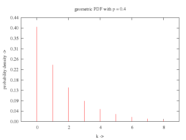
### 22
```ruby
# set title "geometric CDF with p = 0.4"
# set yrange [0 : 1.1]
# set ytics 0, 0.1, 1.0
# plot cgeometric(x, p) with steps
Numo.gnuplot do
set title:"geometric CDF with p = 0.4"
set yrange:0..1.1
set ytics:[0,0.1,1.0]
plot "cgeometric(x, p)", with:"steps"
end
```
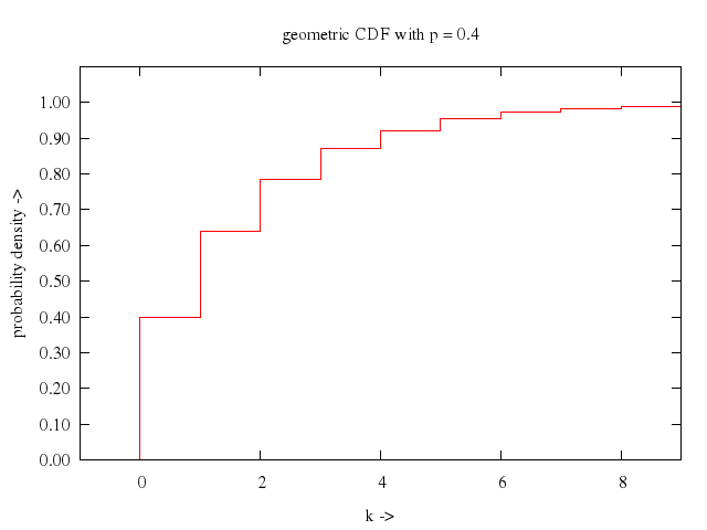
### 23
```ruby
# # Half normal PDF and CDF
# mu = sqrt2invpi
# sigma = 1.0
# s = sigma*sqrt(1.0 - 2.0/pi)
# xmin = -0.2
# xmax = mu + 4.0 * s
# ymax = 1.1 * halfnormal(0, sigma) #Mode of half normal PDF used
# unset key
# set zeroaxis
# set xrange [xmin: xmax]
# set yrange [-0.1: ymax]
# set xlabel "x ->"
# set ylabel "probability density ->"
# set xtics autofreq
# set ytics autofreq
# set format x "%.1f"
# set format y "%.1f"
# set sample 100
# set parametric
# set trange [xmin:xmax]
# set title "half normal PDF, sigma = 1.0"
# set arrow 1 from 0.5,0.13 to 0.0,0.4
# set label 1 "Discontinuity achieved by plotting\ntwice with limited parametric ranges" at 0.2,0.1 left
# plot t<0?t:-eps, halfnormal(t<0?t:-eps, sigma) ls 1, t<0?0.0:t, halfnormal(t<0?0.0:t, sigma) ls 1
Numo.gnuplot do
run "mu = sqrt2invpi"
run "sigma = 1.0"
run "s = sigma*sqrt(1.0 - 2.0/pi)"
run "xmin = -0.2"
run "xmax = mu + 4.0 * s"
run "ymax = 1.1 * halfnormal(0, sigma) #Mode of half normal PDF used"
unset :key
set :zeroaxis
set xrange:"[xmin:xmax]"
set yrange:"[-0.1:ymax]"
set xlabel:"x ->"
set ylabel:"probability density ->"
set xtics:"autofreq"
set ytics:"autofreq"
set format_x:"%.1f"
set format_y:"%.1f"
set sample:100
set :parametric
set trange:"[xmin:xmax]"
set title:"half normal PDF, sigma = 1.0"
set :arrow, 1, from:[0.5,0.13], to:[0.0,0.4]
set :label, 1, "Discontinuity achieved by plotting\ntwice with limited parametric ranges", at:[0.2,0.1], left:true
plot "t<0?t:-eps",
["halfnormal(t<0?t:-eps, sigma)", ls:1],
"t<0?0.0:t",
["halfnormal(t<0?0.0:t, sigma)", ls:1]
end
```
### 24
```ruby
# set title "half normal CDF, sigma = 1.0"
# set yrange [-0.1:1.1]
# set arrow 1 from 0.45,0.1 to 0.05,0.01
# set label 1 "Cusp achieved by plotting twice\nwith limited parametric ranges" at 0.5,0.1 left
# plot t<0?t:-eps, chalfnormal(t<0?t:-eps, sigma) ls 1, t<0?0.0:t, chalfnormal(t<0?0.0:t, sigma) ls 1
Numo.gnuplot do
set title:"half normal CDF, sigma = 1.0"
set yrange:-0.1..1.1
set :arrow, 1, from:[0.45,0.1], to:[0.05,0.01]
set :label, 1, "Cusp achieved by plotting twice\nwith limited parametric ranges", at:[0.5,0.1], left:true
plot "t<0?t:-eps",
["chalfnormal(t<0?t:-eps, sigma)", ls:1],
"t<0?0.0:t",
["chalfnormal(t<0?0.0:t, sigma)", ls:1]
end
```
### 25
```ruby
# unset label 1
# unset arrow 1
# unset parametric
#
# # Hypergeometric PDF and CPF
# N = 75; C = 25; d = 10
# p = real(C) / N
# mu = d * p
# sigma = sqrt(real(N - d) / (N - 1.0) * d * p * (1.0 - p))
# xmin = int(mu - 4.0 * sigma)
# xmin = xmin < -1 ? -1 : xmin
# xmax = int(mu + 4.0 * sigma)
# xmax = xmax < d+1 ? d+1 : xmax
# ymax = 1.1 * hypgeo(int(mu),N,C,d) # approximate mode of hypergeometric PDF used
# unset key
# unset zeroaxis
# set xrange [xmin : xmax]
# set yrange [0 : ymax]
# set xlabel "k ->"
# set ylabel "probability density ->"
# set ytics 0, ymax / 10, ymax
# set format x "%2.0f"
# set format y "%3.2f"
# set sample (xmax - xmin) + 1
# set title "hypergeometric PDF with N = 75, C = 25, d = 10"
# plot hypgeo(x,N,C,d) with impulses
Numo.gnuplot do
unset label:1
unset :arrow, 1
unset :parametric
run "N = 75; C = 25; d = 10"
run "p = real(C) / N"
run "mu = d * p"
run "sigma = sqrt(real(N - d) / (N - 1.0) * d * p * (1.0 - p))"
run "xmin = int(mu - 4.0 * sigma)"
run "xmin = xmin < -1 ? -1 : xmin"
run "xmax = int(mu + 4.0 * sigma)"
run "xmax = xmax < d+1 ? d+1 : xmax"
run "ymax = 1.1 * hypgeo(int(mu),N,C,d) # approximate mode of hypergeometric PDF used"
unset :key
unset :zeroaxis
set xrange:"[xmin:xmax]"
set yrange:"[0:ymax]"
set xlabel:"k ->"
set ylabel:"probability density ->"
set ytics:'0,ymax/10,ymax'
set format_x:"%2.0f"
set format_y:"%3.2f"
set sample:'(xmax - xmin)+1'
set title:"hypergeometric PDF with N = 75, C = 25, d = 10"
plot "hypgeo(x,N,C,d)", with:"impulses"
end
```
### 26
```ruby
# set yrange [0 : 1.1]
# set ytics 0, 1.0 / 10.0, 1.1
# set title "hypergeometric CDF with N = 75, C = 25, d = 10"
# plot chypgeo(x,N,C,d) with steps
Numo.gnuplot do
set yrange:0..1.1
set ytics:'0,1.0/10.0,1.1'
set title:"hypergeometric CDF with N = 75, C = 25, d = 10"
plot "chypgeo(x,N,C,d)", with:"steps"
end
```
### 27
```ruby
# # Laplace PDF
# mu = 0.0; b = 1.0
# sigma = sqrt(2.0) * b
# xmin = mu - 4.0 * sigma
# xmax = mu + 4.0 * sigma
# ymax = 1.1 * laplace(mu, mu, b) #Mode of laplace PDF used
# unset key
# set zeroaxis
# set xrange [xmin: xmax]
# set yrange [0: ymax]
# set xlabel "x ->"
# set ylabel "probability density ->"
# set xtics autofreq
# set ytics autofreq
# set format x "%.1f"
# set format y "%.2f"
# set sample 100+1
# set title "laplace (or double exponential) PDF with mu = 0, b = 1"
# set arrow 1 from -0.95,0.5 to -0.1,0.5
# set label 1 "Cusp achieved by selecting point\nas part of function samples" at -1.0,0.5 right
# plot laplace(x, mu, b)
Numo.gnuplot do
run "mu = 0.0; b = 1.0"
run "sigma = sqrt(2.0) * b"
run "xmin = mu - 4.0 * sigma"
run "xmax = mu + 4.0 * sigma"
run "ymax = 1.1 * laplace(mu, mu, b) #Mode of laplace PDF used"
unset :key
set :zeroaxis
set xrange:"[xmin:xmax]"
set yrange:"[0:ymax]"
set xlabel:"x ->"
set ylabel:"probability density ->"
set xtics:"autofreq"
set ytics:"autofreq"
set format_x:"%.1f"
set format_y:"%.2f"
set sample:'100+1'
set title:"laplace (or double exponential) PDF with mu = 0, b = 1"
set :arrow, 1, from:[-0.95,0.5], to:[-0.1,0.5]
set :label, 1, "Cusp achieved by selecting point\nas part of function samples", at:[-1.0,0.5], right:true
plot "laplace(x, mu, b)"
end
```
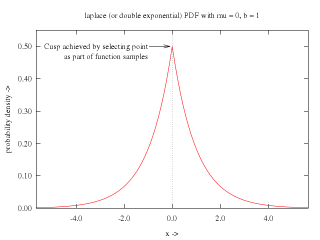
### 28
```ruby
# unset label 1
# unset arrow 1
# set title "laplace (or double exponential) CDF with mu = 0, b = 1"
# set yrange [0: 1.1]
# plot claplace(x, mu, b)
Numo.gnuplot do
unset label:1
unset :arrow, 1
set title:"laplace (or double exponential) CDF with mu = 0, b = 1"
set yrange:0..1.1
plot "claplace(x, mu, b)"
end
```
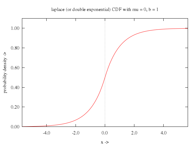
### 29
```ruby
# # Logistic PDF and CDF
# a = 0.0; lambda = 2.0
# mu = a
# sigma = pi / (sqrt(3.0) * lambda)
# xmin = mu - 4.0 * sigma
# xmax = mu + 4.0 * sigma
# ymax = 1.1 * logistic(mu, a, lambda) #Mode of logistic PDF used
# unset key
# set zeroaxis
# set xrange [xmin: xmax]
# set yrange [0: ymax]
# unset key
# set zeroaxis
# set xlabel "x ->"
# set ylabel "probability density ->"
# set xtics autofreq
# set ytics autofreq
# set format x "%.1f"
# set format y "%.1f"
# set sample 100
# set title "logistic PDF with a = 0, lambda = 2"
# plot logistic(x, a, lambda)
Numo.gnuplot do
run "a = 0.0; lambda = 2.0"
run "mu = a"
run "sigma = pi / (sqrt(3.0) * lambda)"
run "xmin = mu - 4.0 * sigma"
run "xmax = mu + 4.0 * sigma"
run "ymax = 1.1 * logistic(mu, a, lambda) #Mode of logistic PDF used"
unset :key
set :zeroaxis
set xrange:"[xmin:xmax]"
set yrange:"[0:ymax]"
unset :key
set :zeroaxis
set xlabel:"x ->"
set ylabel:"probability density ->"
set xtics:"autofreq"
set ytics:"autofreq"
set format_x:"%.1f"
set format_y:"%.1f"
set sample:100
set title:"logistic PDF with a = 0, lambda = 2"
plot "logistic(x, a, lambda)"
end
```
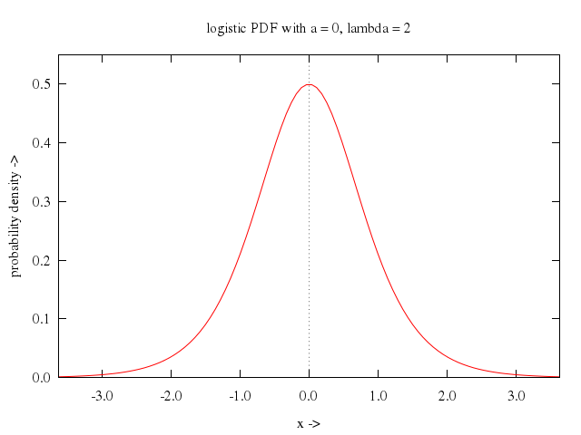
### 30
```ruby
# set title "logistic CDF with a = 0, lambda = 2"
# set yrange [0: 1.1]
# plot clogistic(x, a, lambda)
Numo.gnuplot do
set title:"logistic CDF with a = 0, lambda = 2"
set yrange:0..1.1
plot "clogistic(x, a, lambda)"
end
```
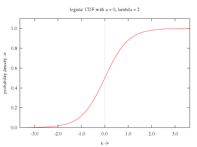
### 31
```ruby
# # Lognormal PDF and CDF
# mu = 1.0; sigma = 0.5
# m = exp(mu + 0.5 * sigma**2)
# s = sqrt(exp(2.0 * mu + sigma**2) * (2.0 * exp(sigma) - 1.0))
# xmin = m - 4.0 * s
# xmin = xmin < 0 ? 0 : xmin
# xmax = m + 4.0 * s
# ymax = 1.1 * lognormal(exp(mu - sigma**2), mu, sigma) #Mode of lognormal PDF used
# unset key
# set zeroaxis
# set xrange [xmin: xmax]
# set yrange [0: ymax]
# set xlabel "x ->"
# set ylabel "probability density ->"
# set xtics autofreq
# set ytics autofreq
# set format x "%.2f"
# set format y "%.2f"
# set sample 100
# set title "lognormal PDF with mu = 1.0, sigma = 0.5"
# plot lognormal(x, mu, sigma)
Numo.gnuplot do
run "mu = 1.0; sigma = 0.5"
run "m = exp(mu + 0.5 * sigma**2)"
run "s = sqrt(exp(2.0 * mu + sigma**2) * (2.0 * exp(sigma) - 1.0))"
run "xmin = m - 4.0 * s"
run "xmin = xmin < 0 ? 0 : xmin"
run "xmax = m + 4.0 * s"
run "ymax = 1.1 * lognormal(exp(mu - sigma**2), mu, sigma) #Mode of lognormal PDF used"
unset :key
set :zeroaxis
set xrange:"[xmin:xmax]"
set yrange:"[0:ymax]"
set xlabel:"x ->"
set ylabel:"probability density ->"
set xtics:"autofreq"
set ytics:"autofreq"
set format_x:"%.2f"
set format_y:"%.2f"
set sample:100
set title:"lognormal PDF with mu = 1.0, sigma = 0.5"
plot "lognormal(x, mu, sigma)"
end
```
### 32
```ruby
# set title "lognormal CDF with mu = 1.0, sigma = 0.5"
# set yrange [0: 1.1]
# plot clognormal(x, mu, sigma)
Numo.gnuplot do
set title:"lognormal CDF with mu = 1.0, sigma = 0.5"
set yrange:0..1.1
plot "clognormal(x, mu, sigma)"
end
```
### 33
```ruby
# # Maxwell PDF
# a = 0.5
# mu = 2.0 / sqrt(pi) / a
# sigma = sqrt(3.0 - 8.0/pi) / a
# xmin = int(mu - 3.0 * sigma)
# xmin = xmin < 0 ? 0 : xmin
# xmax = int(mu + 3.0 * sigma)
# a = 1.5
# ymax = 1.1 * maxwell(1.0 / a, a) + 0.5 #Mode of maxwell PDF used
# ymax = int(ymax + 0.5)
# set zeroaxis
# set xlabel "x ->"
# set ylabel "probability density ->"
# set xtics autofreq
# set ytics autofreq
# set format x "%.1f"
# set format y "%.1f"
# set sample 100
# set title "maxwell PDF"
# set key right top box
# plot [xmin:xmax] [0:ymax] maxwell(x, 1.5) title "a = 1.5", \
# maxwell(x, 1.0) title "a = 1.0", \
# maxwell(x, 0.5) title "a = 0.5"
Numo.gnuplot do
run "a = 0.5"
run "mu = 2.0 / sqrt(pi) / a"
run "sigma = sqrt(3.0 - 8.0/pi) / a"
run "xmin = int(mu - 3.0 * sigma)"
run "xmin = xmin < 0 ? 0 : xmin"
run "xmax = int(mu + 3.0 * sigma)"
run "a = 1.5"
run "ymax = 1.1 * maxwell(1.0 / a, a) + 0.5 #Mode of maxwell PDF used"
run "ymax = int(ymax + 0.5)"
set :zeroaxis
set xlabel:"x ->"
set ylabel:"probability density ->"
set xtics:"autofreq"
set ytics:"autofreq"
set format_x:"%.1f"
set format_y:"%.1f"
set sample:100
set title:"maxwell PDF"
set :key, :right, :top, :box
plot "[xmin:xmax]","[0:ymax]",
["maxwell(x, 1.5)", title:"a = 1.5"],
["maxwell(x, 1.0)", title:"a = 1.0"],
["maxwell(x, 0.5)", title:"a = 0.5"]
end
```
### 34
```ruby
# set title "maxwell CDF"
# set key right bottom box
# plot [xmin:xmax] [0:1.1] cmaxwell(x, 1.5) title "a = 1.5", \
# cmaxwell(x, 1.0) title "a = 1.0", \
# cmaxwell(x, 0.5) title "a = 0.5"
Numo.gnuplot do
set title:"maxwell CDF"
set :key, :right, :bottom, :box
plot "[xmin:xmax]", 0..1.1,
["cmaxwell(x, 1.5)", title:"a = 1.5"],
["cmaxwell(x, 1.0)", title:"a = 1.0"],
["cmaxwell(x, 0.5)", title:"a = 0.5"]
end
```
### 35
```ruby
# # Negative binomial PDF and CDF
# r = 8; p = 0.4
# mu = r * (1.0 - p) / p
# sigma = sqrt(mu / p)
# xmin = int(mu - 4.0 * sigma)
# xmin = xmin < 0 ? 0 : xmin
# xmax = int(mu + 4.0 * sigma)
# ymax = 1.1 * negbin(int(mu - (1.0-p)/p), r, p) #mode of gamma PDF used
# unset key
# unset zeroaxis
# set xrange [xmin-1 : xmax]
# set yrange [0 : ymax]
# set xlabel "k ->"
# set ylabel "probability density ->"
# set ytics 0, ymax / 10, ymax
# set format x "%2.0f"
# set format y "%3.2f"
# set sample (xmax - xmin+1) + 1
# set title "negative binomial (or pascal or polya) PDF with r = 8, p = 0.4"
# plot negbin(x, r, p) with impulses
Numo.gnuplot do
run "r = 8; p = 0.4"
run "mu = r * (1.0 - p) / p"
run "sigma = sqrt(mu / p)"
run "xmin = int(mu - 4.0 * sigma)"
run "xmin = xmin < 0 ? 0 : xmin"
run "xmax = int(mu + 4.0 * sigma)"
run "ymax = 1.1 * negbin(int(mu - (1.0-p)/p), r, p) #mode of gamma PDF used"
unset :key
unset :zeroaxis
set xrange:"[xmin-1:xmax]"
set yrange:"[0:ymax]"
set xlabel:"k ->"
set ylabel:"probability density ->"
set ytics:'0,ymax/10,ymax'
set format_x:"%2.0f"
set format_y:"%3.2f"
set sample:'(xmax - xmin+1)+1'
set title:"negative binomial (or pascal or polya) PDF with r = 8, p = 0.4"
plot "negbin(x, r, p)", with:"impulses"
end
```
### 36
```ruby
# set yrange [0 : 1.1]
# set ytics 0, 0.1, 1.0
# set title "negative binomial (or pascal or polya) CDF with r = 8, p = 0.4"
# plot cnegbin(x, r, p) with steps
Numo.gnuplot do
set yrange:0..1.1
set ytics:[0,0.1,1.0]
set title:"negative binomial (or pascal or polya) CDF with r = 8, p = 0.4"
plot "cnegbin(x, r, p)", with:"steps"
end
```
### 37
```ruby
# # Negative exponential PDF and CDF
# lambda = 2.0
# mu = 1.0 / lambda
# sigma = 1.0 / lambda
# xmax = mu + 4.0 * sigma
# ymax = lambda #No mode
# unset key
# set zeroaxis
# set xrange [0: xmax]
# set yrange [0: ymax]
# set xlabel "x ->"
# set ylabel "probability density ->"
# set xtics autofreq
# set ytics autofreq
# set format x "%.2f"
# set format y "%.1f"
# set sample 100
# set title "negative exponential (or exponential) PDF with lambda = 2.0"
# plot nexp(x, lambda)
Numo.gnuplot do
run "lambda = 2.0"
run "mu = 1.0 / lambda"
run "sigma = 1.0 / lambda"
run "xmax = mu + 4.0 * sigma"
run "ymax = lambda #No mode"
unset :key
set :zeroaxis
set xrange:"[0:xmax]"
set yrange:"[0:ymax]"
set xlabel:"x ->"
set ylabel:"probability density ->"
set xtics:"autofreq"
set ytics:"autofreq"
set format_x:"%.2f"
set format_y:"%.1f"
set sample:100
set title:"negative exponential (or exponential) PDF with lambda = 2.0"
plot "nexp(x, lambda)"
end
```
### 38
```ruby
# set title "negative exponential (or exponential) CDF with lambda = 2.0"
# set yrange [0: 1.1]
# plot cnexp(x, lambda)
Numo.gnuplot do
set title:"negative exponential (or exponential) CDF with lambda = 2.0"
set yrange:0..1.1
plot "cnexp(x, lambda)"
end
```
### 39
```ruby
# # Normal PDF and CDF
# mu = 0.0; sigma = 1.0
# xmin = mu - 4.0 * sigma
# xmax = mu + 4.0 * sigma
# mu = 2.0; sigma = 0.5
# ymax = 1.1 * normal(mu, mu, sigma) #Mode of normal PDF used
# set zeroaxis
# set xlabel "x ->"
# set ylabel "probability density ->"
# set xtics autofreq
# set ytics autofreq
# set format x "%.1f"
# set format y "%.1f"
# set sample 100
# set title "normal (also called gauss or bell-curved) PDF"
# set key left top box
# plot [xmin:xmax] [0:ymax] normal(x, 0, 1.0) title "mu = 0, sigma = 1.0", \
# normal(x, 2, 0.5) title "mu = 2, sigma = 0.5", \
# normal(x, 1, 2.0) title "mu = 1, sigma = 2.0"
Numo.gnuplot do
run "mu = 0.0; sigma = 1.0"
run "xmin = mu - 4.0 * sigma"
run "xmax = mu + 4.0 * sigma"
run "mu = 2.0; sigma = 0.5"
run "ymax = 1.1 * normal(mu, mu, sigma) #Mode of normal PDF used"
set :zeroaxis
set xlabel:"x ->"
set ylabel:"probability density ->"
set xtics:"autofreq"
set ytics:"autofreq"
set format_x:"%.1f"
set format_y:"%.1f"
set sample:100
set title:"normal (also called gauss or bell-curved) PDF"
set :key, :left, :top, :box
plot "[xmin:xmax]","[0:ymax]",
["normal(x, 0, 1.0)", title:"mu = 0, sigma = 1.0"],
["normal(x, 2, 0.5)", title:"mu = 2, sigma = 0.5"],
["normal(x, 1, 2.0)", title:"mu = 1, sigma = 2.0"]
end
```
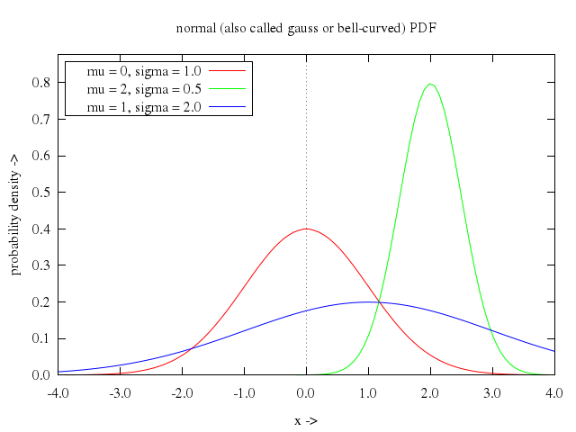
### 40
```ruby
# set title "normal (also called gauss or bell-curved) CDF"
# set key left top box
# plot [xmin:xmax] [0:1.1] mu = 0, sigma = 1.0, cnormal(x, mu, sigma) title "mu = 0, sigma = 1.0", \
# mu = 2, sigma = 0.5, cnormal(x, mu, sigma) title "mu = 2, sigma = 0.5", \
# mu = 1, sigma = 2.0, cnormal(x, mu, sigma) title "mu = 1, sigma = 2.0"
Numo.gnuplot do
set title:"normal (also called gauss or bell-curved) CDF"
set :key, :left, :top, :box
plot "[xmin:xmax]", 0..1.1,
"mu=0",
"sigma=1.0",
["cnormal(x, mu, sigma)", title:"mu = 0, sigma = 1.0"],
"mu=2",
"sigma=0.5",
["cnormal(x, mu, sigma)", title:"mu = 2, sigma = 0.5"],
"mu=1",
"sigma=2.0",
["cnormal(x, mu, sigma)", title:"mu = 1, sigma = 2.0"]
end
```
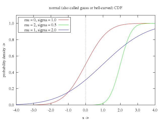
### 41
```ruby
# # Pareto PDF and CDF
# a = 1.0; b = 3.0
# mu = a * b / (b - 1.0)
# sigma = a * sqrt(b) / (sqrt(b - 2.0) * (b - 1.0))
# xmin = mu - 4.0 * sigma
# xmin = xmin < 0 ? 0 : xmin
# xmax = int(mu + 4.0 * sigma)
# ymax = 1.1 * pareto(a, a, b) #mode of pareto PDF used
# ymin = -0.1 * pareto(a, a, b)
# unset key
# set zeroaxis
# set xrange [xmin: xmax]
# set yrange [ymin: ymax]
# set xlabel "x ->"
# set ylabel "probability density ->"
# set xtics autofreq
# set ytics autofreq
# set format x "%.1f"
# set format y "%.1f"
# set sample 200+1
# set title "pareto PDF with a = 1, b = 3"
# # Discontinuity at a
# set parametric
# set trange [0:1-eps]
# x1(t) = -1 + 2*t
# x2(t) = 1 + 3*t
# set arrow 1 from 1.75,0.8 to 1.0,0.8
# set arrow 2 from 1.0,0.0 to 1.0,3.0 nohead lt 0
# set label 1 "Discontinuity achieved by plotting twice\nwith affine mapped parametric ranges" at 1.8,0.8 left
# plot x1(t), pareto(x1(t), a, b) ls 1, x2(t), pareto(x2(t), a, b) ls 1
Numo.gnuplot do
run "a = 1.0; b = 3.0"
run "mu = a * b / (b - 1.0)"
run "sigma = a * sqrt(b) / (sqrt(b - 2.0) * (b - 1.0))"
run "xmin = mu - 4.0 * sigma"
run "xmin = xmin < 0 ? 0 : xmin"
run "xmax = int(mu + 4.0 * sigma)"
run "ymax = 1.1 * pareto(a, a, b) #mode of pareto PDF used"
run "ymin = -0.1 * pareto(a, a, b)"
unset :key
set :zeroaxis
set xrange:"[xmin:xmax]"
set yrange:"[ymin:ymax]"
set xlabel:"x ->"
set ylabel:"probability density ->"
set xtics:"autofreq"
set ytics:"autofreq"
set format_x:"%.1f"
set format_y:"%.1f"
set sample:'200+1'
set title:"pareto PDF with a = 1, b = 3"
set :parametric
set trange:"[0:1-eps]"
run "x1(t) = -1 + 2*t"
run "x2(t) = 1 + 3*t"
set :arrow, 1, from:[1.75,0.8], to:[1.0,0.8]
set :arrow, 2, from:[1.0,0.0], to:[1.0,3.0], nohead:true, lt:0
set :label, 1, "Discontinuity achieved by plotting twice\nwith affine mapped parametric ranges", at:[1.8,0.8], left:true
plot "x1(t)",
["pareto(x1(t), a, b)", ls:1],
"x2(t)",
["pareto(x2(t), a, b)", ls:1]
end
```
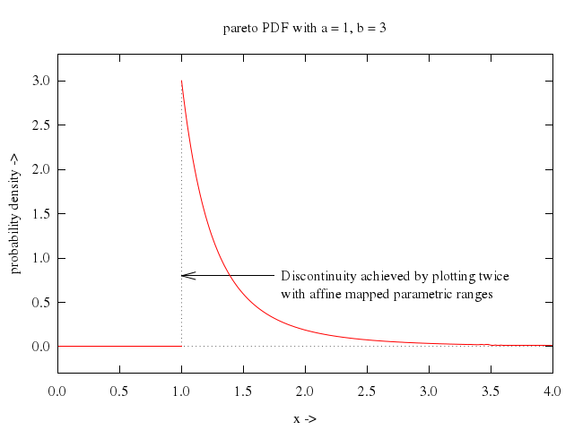
### 42
```ruby
# unset arrow 2
# set title "pareto CDF with a = 1, b = 3"
# unset parametric
# set yrange [-0.1: 1.1]
# set arrow 1 from 1.45,0.1 to 1.05,0.01
# set label 1 "Cusp achieved by selecting point\nas part of function samples" at 1.5,0.1 left
# plot cpareto(x, a, b)
Numo.gnuplot do
unset :arrow, 2
set title:"pareto CDF with a = 1, b = 3"
unset :parametric
set yrange:-0.1..1.1
set :arrow, 1, from:[1.45,0.1], to:[1.05,0.01]
set :label, 1, "Cusp achieved by selecting point\nas part of function samples", at:[1.5,0.1], left:true
plot "cpareto(x, a, b)"
end
```
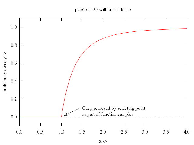
### 43
```ruby
# unset label 1
# unset arrow 1
#
# # Poisson PDF and CDF
# mu = 4.0
# sigma = sqrt(mu)
# xmin = int(mu - 4.0 * sigma)
# xmin = xmin < -1 ? -1 : xmin
# xmax = int(mu + 4.0 * sigma)
# ymax = 1.1 * poisson(mu, mu) #mode of poisson PDF used
# unset key
# set zeroaxis
# set xrange [xmin : xmax]
# set yrange [0 : ymax]
# set xlabel "k ->"
# set ylabel "probability density ->"
# set ytics 0, ymax / 10, ymax
# set format x "%2.0f"
# set format y "%3.2f"
# set sample (xmax - xmin) + 1
# set title "poisson PDF with mu = 4.0"
# plot poisson(x, mu) with impulses
Numo.gnuplot do
unset label:1
unset :arrow, 1
run "mu = 4.0"
run "sigma = sqrt(mu)"
run "xmin = int(mu - 4.0 * sigma)"
run "xmin = xmin < -1 ? -1 : xmin"
run "xmax = int(mu + 4.0 * sigma)"
run "ymax = 1.1 * poisson(mu, mu) #mode of poisson PDF used"
unset :key
set :zeroaxis
set xrange:"[xmin:xmax]"
set yrange:"[0:ymax]"
set xlabel:"k ->"
set ylabel:"probability density ->"
set ytics:'0,ymax/10,ymax'
set format_x:"%2.0f"
set format_y:"%3.2f"
set sample:'(xmax - xmin)+1'
set title:"poisson PDF with mu = 4.0"
plot "poisson(x, mu)", with:"impulses"
end
```
### 44
```ruby
# set yrange [-0.1 : 1.1]
# set ytics -0.1, 0.1, 1.1
# set title "poisson CDF with mu = 4.0"
# plot cpoisson(x, mu) with steps
Numo.gnuplot do
set yrange:-0.1..1.1
set ytics:[-0.1,0.1,1.1]
set title:"poisson CDF with mu = 4.0"
plot "cpoisson(x, mu)", with:"steps"
end
```
### 45
```ruby
# # Rayleigh PDF and CDF
# lambda = 2.0
# mu = 0.5 * sqrt(pi / lambda)
# sigma = sqrt((1.0 - pi / 4.0) / lambda)
# xmax = mu + 4.0 * sigma
# ymax = 1.1 * rayleigh(1.0 / sqrt(2.0 * lambda), lambda) #Mode of rayleigh PDF used
# unset key
# set zeroaxis
# set xrange [0: xmax]
# set yrange [0: ymax]
# set xlabel "x ->"
# set ylabel "probability density ->"
# set xtics autofreq
# set ytics autofreq
# set format x "%.2f"
# set format y "%.1f"
# set sample 100
# set title "rayleigh PDF with lambda = 2.0"
# plot rayleigh(x, lambda)
Numo.gnuplot do
run "lambda = 2.0"
run "mu = 0.5 * sqrt(pi / lambda)"
run "sigma = sqrt((1.0 - pi / 4.0) / lambda)"
run "xmax = mu + 4.0 * sigma"
run "ymax = 1.1 * rayleigh(1.0 / sqrt(2.0 * lambda), lambda) #Mode of rayleigh PDF used"
unset :key
set :zeroaxis
set xrange:"[0:xmax]"
set yrange:"[0:ymax]"
set xlabel:"x ->"
set ylabel:"probability density ->"
set xtics:"autofreq"
set ytics:"autofreq"
set format_x:"%.2f"
set format_y:"%.1f"
set sample:100
set title:"rayleigh PDF with lambda = 2.0"
plot "rayleigh(x, lambda)"
end
```
### 46
```ruby
# set title "rayleigh CDF with lambda = 2.0"
# set yrange [0: 1.1]
# plot crayleigh(x, lambda)
Numo.gnuplot do
set title:"rayleigh CDF with lambda = 2.0"
set yrange:0..1.1
plot "crayleigh(x, lambda)"
end
```
### 47
```ruby
# # Sine PDF and CDF
# a = 3.2; f = 2.6
# mu = a / 2.0
# sigma = sqrt(a * a / 3.0 * (1.0 - 3.0 / (2.0 * n * n * pi * pi)) - mu * mu)
# xmin = 0.0
# xmax = a - eps
# a = 2; f = 1.0
# ymax = 1.1 * 2.0 / a #Mode of sine PDF used
# set zeroaxis
# set xlabel "x ->"
# set ylabel "probability density ->"
# set xtics autofreq
# set ytics autofreq
# set format x "%.2f"
# set format y "%.1f"
# set sample 250
# set title "sine PDF"
# set key bottom outside
# keystr(a, f) = sprintf("a = %0.1f, f = %0.1f", a, f)
# a1 = 2.0; a2 = 3.25; a3 = 2.75
# f1 = 1.0; f2 = 3.0; f3 = 2.6; f4 = 0.0
# plot [xmin:xmax] [0:ymax] a = a1, f = f1, sine(x, f, a) title keystr(a, f), \
# a = a1, f = f2, sine(x, f, a) title keystr(a, f), \
# a = a2, f = f3, sine(x, f, a) title keystr(a, f), \
# a = a3, f = f4, sine(x, f, a) title keystr(a, f) with steps
Numo.gnuplot do
run "a = 3.2; f = 2.6"
run "mu = a / 2.0"
run "sigma = sqrt(a * a / 3.0 * (1.0 - 3.0 / (2.0 * n * n * pi * pi)) - mu * mu)"
run "xmin = 0.0"
run "xmax = a - eps"
run "a = 2; f = 1.0"
run "ymax = 1.1 * 2.0 / a #Mode of sine PDF used"
set :zeroaxis
set xlabel:"x ->"
set ylabel:"probability density ->"
set xtics:"autofreq"
set ytics:"autofreq"
set format_x:"%.2f"
set format_y:"%.1f"
set sample:250
set title:"sine PDF"
set :key, :bottom, :outside
run "keystr(a, f) = sprintf(\"a = %0.1f, f = %0.1f\", a, f)"
run "a1 = 2.0; a2 = 3.25; a3 = 2.75"
run "f1 = 1.0; f2 = 3.0; f3 = 2.6; f4 = 0.0"
plot "[xmin:xmax]","[0:ymax]",
"a=a1",
"f=f1",
["sine(x, f, a)", title_nq:'keystr(a, f)'],
"a=a1",
"f=f2",
["sine(x, f, a)", title_nq:'keystr(a, f)'],
"a=a2",
"f=f3",
["sine(x, f, a)", title_nq:'keystr(a, f)'],
"a=a3",
"f=f4",
["sine(x, f, a)", title_nq:'keystr(a, f)', with:"steps"]
end
```
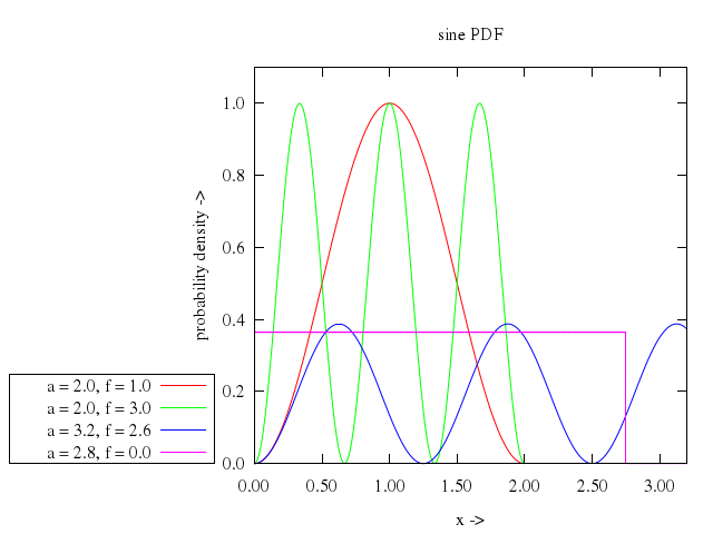
### 48
```ruby
# set title "sine CDF"
# set key top left
# plot [xmin:xmax] [0:1.1] a = a1, f = f1, csine(x, f, a) title keystr(a, f), \
# a = a1, f = f2, csine(x, f, a) title keystr(a, f), \
# a = a2, f = f3, csine(x, f, a) title keystr(a, f), \
# a = a3, f = f4, csine(x, f, a) title keystr(a, f) with steps
Numo.gnuplot do
set title:"sine CDF"
set :key, :top, :left
plot "[xmin:xmax]", 0..1.1,
"a=a1",
"f=f1",
["csine(x, f, a)", title_nq:'keystr(a, f)'],
"a=a1",
"f=f2",
["csine(x, f, a)", title_nq:'keystr(a, f)'],
"a=a2",
"f=f3",
["csine(x, f, a)", title_nq:'keystr(a, f)'],
"a=a3",
"f=f4",
["csine(x, f, a)", title_nq:'keystr(a, f)', with:"steps"]
end
```
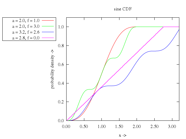
### 49
```ruby
# # t PDF and CDF
# nu = 20
# mu = 0
# sigma = nu > 2 ? sqrt(nu / (nu - 2.0)) : 1.0
# xmin = mu - 4.0 * sigma
# xmax = mu + 4.0 * sigma
# ymax = 1.1 * t(mu, nu) #Mode of t PDF used
# set key inside center left title "degrees of freedom"
# set zeroaxis
# set xrange [xmin: xmax]
# set yrange [0: ymax]
# set xlabel "x ->"
# set ylabel "probability density ->"
# set xtics autofreq
# set ytics autofreq
# set format x "%.1f"
# set format y "%.2f"
# set sample 100
# set title "t PDF (and Gaussian limit)"
# ks(nu) = sprintf("nu = %d", nu)
# plot t(x, 1) ti ks(1), t(x, 2) ti ks(2), t(x, 4) ti ks(4), t(x, 10) ti ks(10), \
# t(x, 20) ti ks(20), normal(x, 0, 1) ti "normal"
Numo.gnuplot do
run "nu = 20"
run "mu = 0"
run "sigma = nu > 2 ? sqrt(nu / (nu - 2.0)) : 1.0"
run "xmin = mu - 4.0 * sigma"
run "xmax = mu + 4.0 * sigma"
run "ymax = 1.1 * t(mu, nu) #Mode of t PDF used"
set :key, :inside, :center, :left, title:"degrees of freedom"
set :zeroaxis
set xrange:"[xmin:xmax]"
set yrange:"[0:ymax]"
set xlabel:"x ->"
set ylabel:"probability density ->"
set xtics:"autofreq"
set ytics:"autofreq"
set format_x:"%.1f"
set format_y:"%.2f"
set sample:100
set title:"t PDF (and Gaussian limit)"
run "ks(nu) = sprintf(\"nu = %d\", nu)"
plot ["t(x, 1)", ti_nq:'ks(1)'],
["t(x, 2)", ti_nq:'ks(2)'],
["t(x, 4)", ti_nq:'ks(4)'],
["t(x, 10)", ti_nq:'ks(10)'],
["t(x, 20)", ti_nq:'ks(20)'],
["normal(x, 0, 1)", ti:"normal"]
end
```
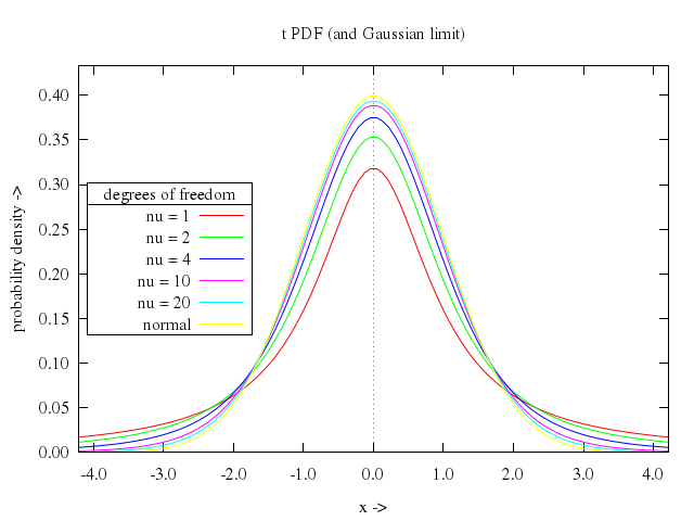
### 50
```ruby
# set title "t CDF (and Gaussian limit)"
# set yrange [0: 1.1]
# plot ct(x, 1) ti ks(1), ct(x, 2) ti ks(2), ct(x, 4) ti ks(4), ct(x, 10) ti ks(10), \
# ct(x, 20) ti ks(20), cnormal(x, 0, 1) ti "normal"
Numo.gnuplot do
set title:"t CDF (and Gaussian limit)"
set yrange:0..1.1
plot ["ct(x, 1)", ti_nq:'ks(1)'],
["ct(x, 2)", ti_nq:'ks(2)'],
["ct(x, 4)", ti_nq:'ks(4)'],
["ct(x, 10)", ti_nq:'ks(10)'],
["ct(x, 20)", ti_nq:'ks(20)'],
["cnormal(x, 0, 1)", ti:"normal"]
end
```
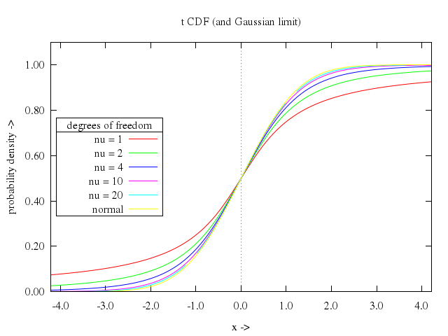
### 51
```ruby
# # Thanks to [email protected] for telling us about this
# # triangular PDF and CDF
# m = 3.0
# g = 2.0
# mu = m
# sigma = g/sqrt(6.0)
# xmin = m - 1.1*g
# xmax = m + 1.1*g
# ymax = 1.1 * triangular(m, m, g) #Mode of triangular PDF used
# ymin = -ymax/11.0;
# unset key
# set zeroaxis
# set xrange [xmin: xmax]
# set yrange [ymin: ymax]
# set xlabel "x ->"
# set ylabel "probability density ->"
# set xtics autofreq
# set ytics autofreq
# set format x "%.1f"
# set format y "%.2f"
# set sample 50*1.1*g+1
# set title "triangular PDF with m = 3.0, g = 2.0"
# plot triangular(x, m, g)
Numo.gnuplot do
run "m = 3.0"
run "g = 2.0"
run "mu = m"
run "sigma = g/sqrt(6.0)"
run "xmin = m - 1.1*g"
run "xmax = m + 1.1*g"
run "ymax = 1.1 * triangular(m, m, g) #Mode of triangular PDF used"
run "ymin = -ymax/11.0;"
unset :key
set :zeroaxis
set xrange:"[xmin:xmax]"
set yrange:"[ymin:ymax]"
set xlabel:"x ->"
set ylabel:"probability density ->"
set xtics:"autofreq"
set ytics:"autofreq"
set format_x:"%.1f"
set format_y:"%.2f"
set sample:'50*1.1*g+1'
set title:"triangular PDF with m = 3.0, g = 2.0"
plot "triangular(x, m, g)"
end
```
### 52
```ruby
# set title "triangular CDF with m = 3.0, g = 2.0"
# set yrange [-0.1: 1.1]
# plot ctriangular(x, m, g)
Numo.gnuplot do
set title:"triangular CDF with m = 3.0, g = 2.0"
set yrange:-0.1..1.1
plot "ctriangular(x, m, g)"
end
```
### 53
```ruby
# # Uniform PDF and CDF
# a = -2.0; b= 2.0
# mu = (a + b) / 2.0
# sigma = (b - a) / sqrt(12.0)
# xmin = a - 0.1*(b - a)
# xmax = b + 0.1*(b - a)
# ymax = 1.1 * uniform(mu, a, b) #No mode
# ymin = -0.1 * uniform(mu, a, b)
# unset key
# set zeroaxis
# set xrange [xmin: xmax]
# set yrange [ymin: ymax]
# set xlabel "x ->"
# set ylabel "probability density ->"
# set xtics autofreq
# set ytics autofreq
# set format x "%.2f"
# set format y "%.2f"
# set sample 120+1
# set title "uniform PDF with a = -2.0, b = 2.0"
# plot uniform(x, a, b) with steps
Numo.gnuplot do
run "a = -2.0; b= 2.0"
run "mu = (a + b) / 2.0"
run "sigma = (b - a) / sqrt(12.0)"
run "xmin = a - 0.1*(b - a)"
run "xmax = b + 0.1*(b - a)"
run "ymax = 1.1 * uniform(mu, a, b) #No mode"
run "ymin = -0.1 * uniform(mu, a, b)"
unset :key
set :zeroaxis
set xrange:"[xmin:xmax]"
set yrange:"[ymin:ymax]"
set xlabel:"x ->"
set ylabel:"probability density ->"
set xtics:"autofreq"
set ytics:"autofreq"
set format_x:"%.2f"
set format_y:"%.2f"
set sample:'120+1'
set title:"uniform PDF with a = -2.0, b = 2.0"
plot "uniform(x, a, b)", with:"steps"
end
```
### 54
```ruby
# set title "uniform CDF with a = -2.0, b = 2.0"
# set yrange [-0.1 : 1.1]
# plot cuniform(x, a, b)
Numo.gnuplot do
set title:"uniform CDF with a = -2.0, b = 2.0"
set yrange:-0.1..1.1
plot "cuniform(x, a, b)"
end
```
### 55
```ruby
# # Weibull PDF and CDF
# lambda = 1.0/5; a = 1.0
# mu = 1.0 / lambda * gamma(1.0 / a) / a
# sigma = sqrt(lambda**(-2.0) * (2.0 * gamma(2.0 / a) / a - (gamma(1.0 / a) / a)**2))
# xmin = mu - 4.0 * sigma
# xmin = xmin < 0 ? 0 : xmin
# #Mode of weibull PDF used
# ymax = 1.8 * (a >= 1.0 ? weibull(((a - 1.0) / a)**(1.0 / a) / lambda, a, lambda) : 2.0)
# lambda = 1.0/15; a = 10.0
# mu = 1.0 / lambda * gamma(1.0 / a) / a
# sigma = sqrt(lambda**(-2.0) * (2.0 * gamma(2.0 / a) / a - (gamma(1.0 / a) / a)**2))
# xmax = int(mu + 4.0 * sigma)
# set key on title "" inside top right
# set zeroaxis
# set grid
# set xrange [xmin : xmax]
# set xlabel "x ->"
# set ylabel "probability density ->"
# set xtics autofreq
# set ytics autofreq
# set format x "%g"
# set format y "%g"
# set sample 100
# set title "weibull PDF"
# ks(a,lambda) = sprintf("lambda = 1/%g, a = %0.1f", 1.0/lambda, a)
# a1 = 0.5; a2 = 1.0; a3 = 2.0; a4 = 10.0
# lambda1 = 1.0/5; lambda2 = 1.0/15
# set arrow 1 from 3.8,0.27 to 0.5,weibull(0.5,a1,lambda1)
# set label 1 "a < 1, rate descreasing over time" at 4,0.27 left
# set arrow 2 from 8,0.19 to 6.4,weibull(6.4,a3,lambda1)
# set arrow 3 from 10.5,0.19 to 13,weibull(13,a4,lambda2)
# set label 2 "a > 1, rate increasing over time" at 9,0.2 center
# plot [] [0:ymax] lambda = lambda1, a = a1, weibull(x, a, lambda) ti ks(a, lambda), \
# lambda = lambda1, a = a2, weibull(x, a, lambda) ti ks(a, lambda), \
# lambda = lambda1, a = a3, weibull(x, a, lambda) ti ks(a, lambda), \
# lambda = lambda2, a = a4, weibull(x, a, lambda) ti ks(a, lambda)
Numo.gnuplot do
run "lambda = 1.0/5; a = 1.0"
run "mu = 1.0 / lambda * gamma(1.0 / a) / a"
run "sigma = sqrt(lambda**(-2.0) * (2.0 * gamma(2.0 / a) / a - (gamma(1.0 / a) / a)**2))"
run "xmin = mu - 4.0 * sigma"
run "xmin = xmin < 0 ? 0 : xmin"
run "ymax = 1.8 * (a >= 1.0 ? weibull(((a - 1.0) / a)**(1.0 / a) / lambda, a, lambda) : 2.0)"
run "lambda = 1.0/15; a = 10.0"
run "mu = 1.0 / lambda * gamma(1.0 / a) / a"
run "sigma = sqrt(lambda**(-2.0) * (2.0 * gamma(2.0 / a) / a - (gamma(1.0 / a) / a)**2))"
run "xmax = int(mu + 4.0 * sigma)"
set :key, :on, title:"", inside:true, top:true, right:true
set :zeroaxis
set :grid
set xrange:"[xmin:xmax]"
set xlabel:"x ->"
set ylabel:"probability density ->"
set xtics:"autofreq"
set ytics:"autofreq"
set format_x:"%g"
set format_y:"%g"
set sample:100
set title:"weibull PDF"
run "ks(a,lambda) = sprintf(\"lambda = 1/%g, a = %0.1f\", 1.0/lambda, a)"
run "a1 = 0.5; a2 = 1.0; a3 = 2.0; a4 = 10.0"
run "lambda1 = 1.0/5; lambda2 = 1.0/15"
set :arrow, 1, from:[3.8,0.27], to:"0.5,weibull(0.5,a1,lambda1)"
set :label, 1, "a < 1, rate descreasing over time", at:[4,0.27], left:true
set :arrow, 2, from:[8,0.19], to:"6.4,weibull(6.4,a3,lambda1)"
set :arrow, 3, from:[10.5,0.19], to:"13,weibull(13,a4,lambda2)"
set :label, 2, "a > 1, rate increasing over time", at:[9,0.2], center:true
plot "[]","[0:ymax]",
"lambda=lambda1",
"a=a1",
["weibull(x, a, lambda)", ti_nq:'ks(a, lambda)'],
"lambda=lambda1",
"a=a2",
["weibull(x, a, lambda)", ti_nq:'ks(a, lambda)'],
"lambda=lambda1",
"a=a3",
["weibull(x, a, lambda)", ti_nq:'ks(a, lambda)'],
"lambda=lambda2",
"a=a4",
["weibull(x, a, lambda)", ti_nq:'ks(a, lambda)']
end
```
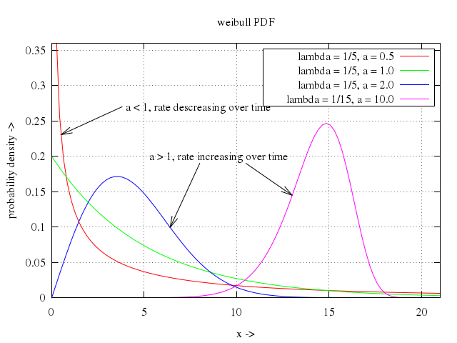
### 56
```ruby
# unset label 1; unset label 2
# unset arrow 1; unset arrow 2; unset arrow 3
# set key at 9,0.4 center
# set title "weibull CDF"
# plot [] [0:1.1] lambda = lambda1, a = a1, cweibull(x, a, lambda) ti ks(a, lambda), \
# lambda = lambda1, a = a2, cweibull(x, a, lambda) ti ks(a, lambda), \
# lambda = lambda1, a = a3, cweibull(x, a, lambda) ti ks(a, lambda), \
# lambda = lambda2, a = a4, cweibull(x, a, lambda) ti ks(a, lambda)
Numo.gnuplot do
unset label:1; unset label:2
unset :arrow, 1; unset :arrow, 2; unset :arrow, 3
set :key, at:[9,0.4], center:true
set title:"weibull CDF"
plot "[]", 0..1.1,
"lambda=lambda1",
"a=a1",
["cweibull(x, a, lambda)", ti_nq:'ks(a, lambda)'],
"lambda=lambda1",
"a=a2",
["cweibull(x, a, lambda)", ti_nq:'ks(a, lambda)'],
"lambda=lambda1",
"a=a3",
["cweibull(x, a, lambda)", ti_nq:'ks(a, lambda)'],
"lambda=lambda2",
"a=a4",
["cweibull(x, a, lambda)", ti_nq:'ks(a, lambda)']
end
```
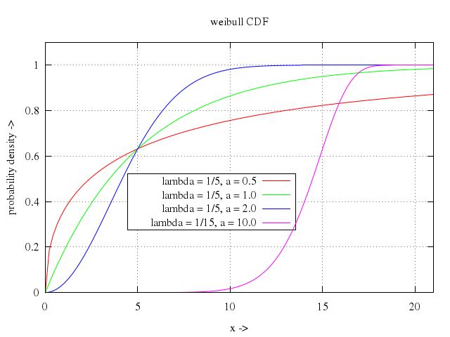
## random numbers
[Original Demo](http://gnuplot.sourceforge.net/demo_4.6/random.html)
### 1
```ruby
# # random.dem
# #
# # Lattice test for random numbers;
# # If you can see any patterns in this plot, the random number generator
# # is not very good.
# #
# # Copyright (c) 1991, Jos van der Woude, [email protected]
#
# # History:
# # - 6. 6. 2006 ds: added univariate and multivariate normal example
# # - 10. 5. 2006 ds: added univariate and multivariate normal example
# # - ?. ? 1991 jvdw: 1st version
#
# unset key
# set xrange [0: 1]
# set yrange [0: 1]
# set zrange [0: 1]
# set title "Lattice test for random numbers"
# set xlabel "rand(n) ->"
# set ylabel "rand(n + 1) ->"
# set zlabel "rand(n + 2) ->"
# set format x "%3.2f"
# set format y "%3.2f"
# set format z "%3.2f"
# set tics
# set sample 1000
# set style function dots
# set parametric
# plot rand(0), rand(0)
Numo.gnuplot do
unset :key
set xrange:0..1
set yrange:0..1
set zrange:0..1
set title:"Lattice test for random numbers"
set xlabel:"rand(n) ->"
set ylabel:"rand(n + 1) ->"
set zlabel:"rand(n + 2) ->"
set format_x:"%3.2f"
set format_y:"%3.2f"
set format_z:"%3.2f"
set :tics
set sample:1000
set :style, :function, :dots
set :parametric
plot "rand(0)",
"rand(0)"
end
```
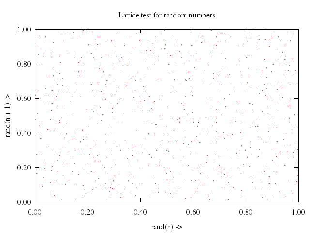
### 2
```ruby
# print "3D plot ahead, one moment please ..."
# set sample 50
# splot rand(0), rand(0), rand(0)
Numo.gnuplot do
set sample:50
splot "rand(0)",
"rand(0)",
"rand(0)"
end
```
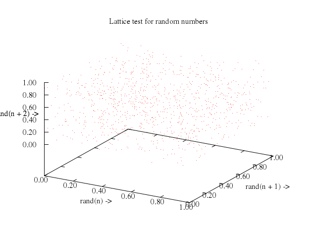
### 3
```ruby
# print ""
# print "Multivariate normal distribution"
# print ""
# print "The surface plot shows a two variable multivariate probability"
# print "density function. On the x-y plane are some samples of the random"
# print "vector and a contour plot illustrating the correlation, which in"
# print "this case is zero, i.e. a circle. (Easier to view in map mode.)"
# print ""
# nsamp = 50
# # Generate N random data points.
# set print "random.tmp"
# do for [i=1:nsamp] {
# print sprintf("%8.5g %8.5g", invnorm(rand(0)), invnorm(rand(0)))
# }
# unset print
# #
# unset xlabel
# unset ylabel
# unset zlabel
# set parametric
# tstring(n) = sprintf("%d random samples from a 2D Gaussian PDF with\nunit variance, zero mean and no dependence", n)
# set title tstring(nsamp)
# unset key
# set hidden3d
# #set dgrid3d
# set contour
# set view 68, 28, 1, 1
# set cntrparam levels discrete 0.1
# unset clabel
# set xrange [-3:3]
# set yrange [-3:3]
# set zrange [-0.2:0.2]
# set ztics 0,0.05
# set urange [-3:3]
# set vrange [-3:3]
# set ticslevel 0
# set isosamples 30
# splot u,v,( 1/(2*pi) * exp(-0.5 * (u**2 + v**2)) ) with line lc rgb "black", \
# "random.tmp" using 1:2:(-0.2) with points pointtype 7 lc rgb "black"
Numo.gnuplot do
run "nsamp = 50"
run <0)?int1a(x,x/ceil(x/delta)):-int1b(x,-x/ceil(-x/delta))
# int1a(x,d) = (x<=d*.1) ? 0 : (int1a(x-d,d)+(f(x-d)+4*f(x-d*.5)+f(x))*d/6.)
# int1b(x,d) = (x>=-d*.1) ? 0 : (int1b(x+d,d)+(f(x+d)+4*f(x+d*.5)+f(x))*d/6.)
# #
# # integral2_f(x,y) takes two variables; x is the lower limit, and y the upper.
# # calculate the integral of function f(t) from x to y
# integral2_f(x,y) = (xy-d*.5) ? 0 : (int2(x+d,y,d) + (f(x)+4*f(x+d*.5)+f(x+d))*d/6.)
#
# set autoscale
# set title "approximate the integral of functions"
# set samples 50
# set key bottom right
#
# f(x) = exp(-x**2)
#
# plot [-5:5] f(x) title "f(x)=exp(-x**2)", \
# 2/sqrt(pi)*integral_f(x) title "erf(x)=2/sqrt(pi)*integral_f(x)", \
# erf(x) with points
Numo.gnuplot do
run "delta = 0.2"
run "integral_f(x) = (x>0)?int1a(x,x/ceil(x/delta)):-int1b(x,-x/ceil(-x/delta))"
run "int1a(x,d) = (x<=d*.1) ? 0 : (int1a(x-d,d)+(f(x-d)+4*f(x-d*.5)+f(x))*d/6.)"
run "int1b(x,d) = (x>=-d*.1) ? 0 : (int1b(x+d,d)+(f(x+d)+4*f(x+d*.5)+f(x))*d/6.)"
run "integral2_f(x,y) = (xy-d*.5) ? 0 : (int2(x+d,y,d) + (f(x)+4*f(x+d*.5)+f(x+d))*d/6.)"
set :autoscale
set title:"approximate the integral of functions"
set samples:50
set :key, :bottom, :right
run "f(x) = exp(-x**2)"
plot -5..5,
["f(x)", title:"f(x)=exp(-x**2)"],
["2/sqrt(pi)*integral_f(x)", title:"erf(x)=2/sqrt(pi)*integral_f(x)"],
["erf(x)", with:"points"]
end
```
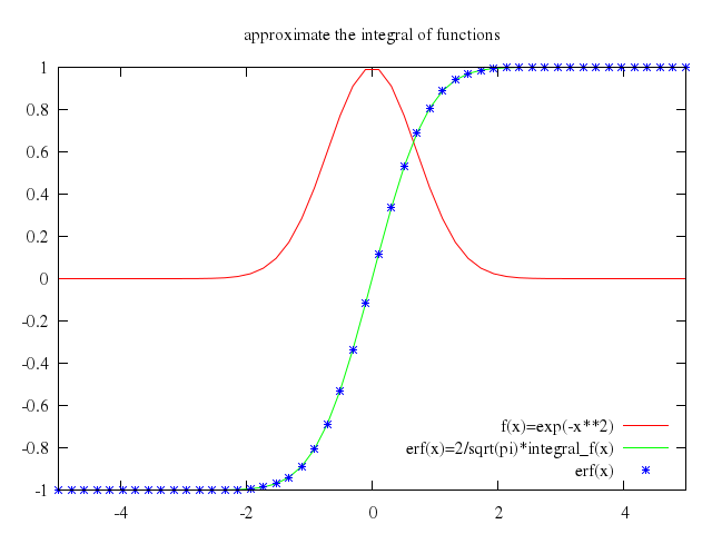
### 2
```ruby
# f(x)=cos(x)
#
# plot [-5:5] f(x) title "f(x)=cos(x)", integral_f(x)
Numo.gnuplot do
run "f(x)=cos(x)"
plot -5..5,
["f(x)", title:"f(x)=cos(x)"],
"integral_f(x)"
end
```
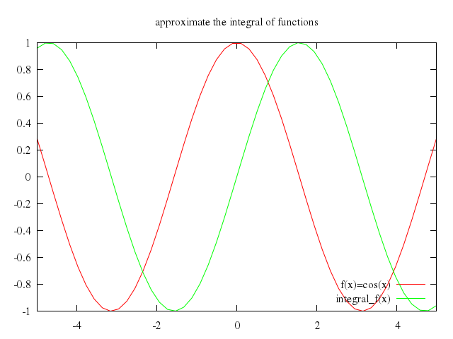
### 3
```ruby
# set title "approximate the integral of functions (upper and lower limits)"
#
# f(x)=(x-2)**2-20
#
# plot [-10:10] f(x) title "f(x)=(x-2)**2-20", integral2_f(-5,x)
Numo.gnuplot do
set title:"approximate the integral of functions (upper and lower limits)"
run "f(x)=(x-2)**2-20"
plot -10..10,
["f(x)", title:"f(x)=(x-2)**2-20"],
"integral2_f(-5,x)"
end
```
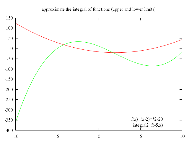
### 4
```ruby
# f(x)=sin(x-1)-.75*sin(2*x-1)+(x**2)/8-5
#
# plot [-10:10] f(x) title "f(x)=sin(x-1)-0.75*sin(2*x-1)+(x**2)/8-5", integral2_f(x,1)
Numo.gnuplot do
run "f(x)=sin(x-1)-.75*sin(2*x-1)+(x**2)/8-5"
plot -10..10,
["f(x)", title:"f(x)=sin(x-1)-0.75*sin(2*x-1)+(x**2)/8-5"],
"integral2_f(x,1)"
end
```
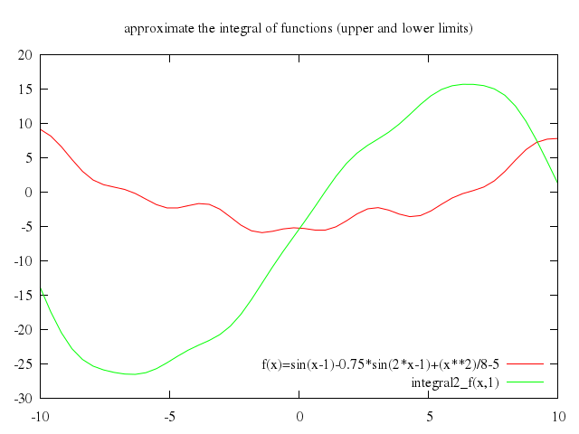
### 5
```ruby
# # This definition computes the ackermann. Do not attempt to compute its
# # values for non integral values. In addition, do not attempt to compute
# # its beyond m = 3, unless you want to wait really long time.
#
# ack(m,n) = (m == 0) ? n + 1 : (n == 0) ? ack(m-1,1) : ack(m-1,ack(m,n-1))
#
# set xrange [0:3]
# set yrange [0:3]
#
# set isosamples 4
# set samples 4
#
# set title "Plot of the ackermann function"
#
# splot ack(x, y)
Numo.gnuplot do
run "ack(m,n) = (m == 0) ? n + 1 : (n == 0) ? ack(m-1,1) : ack(m-1,ack(m,n-1))"
set xrange:0..3
set yrange:0..3
set isosamples:4
set samples:4
set title:"Plot of the ackermann function"
splot "ack(x, y)"
end
```
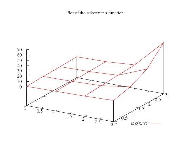
### 6
```ruby
# set xrange [-5:5]
# set yrange [-10:10]
# set isosamples 10
# set samples 100
# set key top right at 4,-3
# set title "Min(x,y) and Max(x,y)"
#
# #
# min(x,y) = (x < y) ? x : y
# max(x,y) = (x > y) ? x : y
#
# plot sin(x), x**2, x**3, max(sin(x), min(x**2, x**3))+0.5
Numo.gnuplot do
set xrange:-5..5
set yrange:-10..10
set isosamples:10
set samples:100
set :key, :top, :right, at:[4,-3]
set title:"Min(x,y) and Max(x,y)"
run "min(x,y) = (x < y) ? x : y"
run "max(x,y) = (x > y) ? x : y"
plot "sin(x)",
"x**2",
"x**3",
"max(sin(x), min(x**2, x**3))+0.5"
end
```
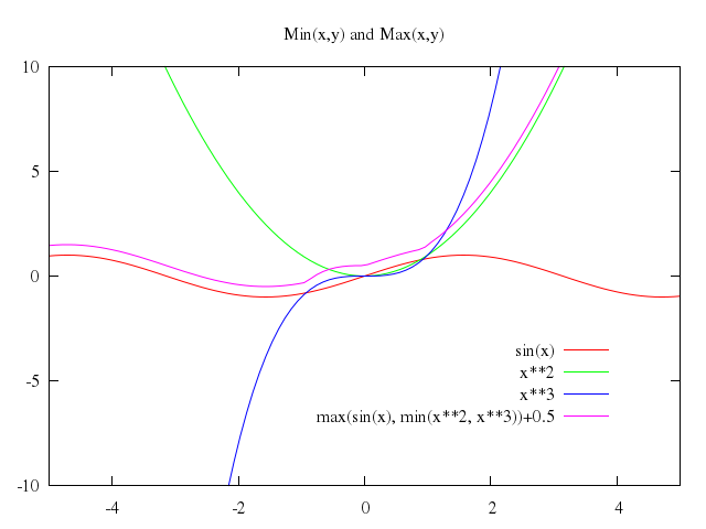
### 7
```ruby
# # gcd(x,y) finds the greatest common divisor of x and y,
# # using Euclid's algorithm
# # as this is defined only for integers, first round to the nearest integer
# gcd(x,y) = gcd1(rnd(max(x,y)),rnd(min(x,y)))
# gcd1(x,y) = (y == 0) ? x : gcd1(y, x - x/y * y)
# rnd(x) = int(x+0.5)
#
# set samples 59
# set xrange [1:59]
# set auto
# set key default
#
# set title "Greatest Common Divisor (for integers only)"
#
# plot gcd(x, 60) with impulses
Numo.gnuplot do
run "gcd(x,y) = gcd1(rnd(max(x,y)),rnd(min(x,y)))"
run "gcd1(x,y) = (y == 0) ? x : gcd1(y, x - x/y * y)"
run "rnd(x) = int(x+0.5)"
set samples:59
set xrange:1..59
set :auto
set :key, :default
set title:"Greatest Common Divisor (for integers only)"
plot "gcd(x, 60)", with:"impulses"
end
```
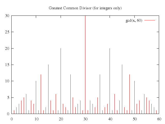
### 8
```ruby
# # This definition computes the sum of the first 10, 100, 1000 fourier
# # coefficients of a (particular) square wave.
#
# set title "Finite summation of 10, 100, 1000 fourier coefficients"
#
# set samples 500
# set xrange [-10:10]
# set yrange [-0.4:1.2]
# set key bottom right
#
# fourier(k, x) = sin(3./2*k)/k * 2./3*cos(k*x)
# sum10(x) = 1./2 + sum [k=1:10] fourier(k, x)
# sum100(x) = 1./2 + sum [k=1:100] fourier(k, x)
# sum1000(x) = 1./2 + sum [k=1:1000] fourier(k, x)
#
# plot \
# sum10(x) title "1./2 + sum [k=1:10] sin(3./2*k)/k * 2./3*cos(k*x)", \
# sum100(x) title "1./2 + sum [k=1:100] sin(3./2*k)/k * 2./3*cos(k*x)", \
# sum1000(x) title "1./2 + sum [k=1:1000] sin(3./2*k)/k * 2./3*cos(k*x)"
Numo.gnuplot do
set title:"Finite summation of 10, 100, 1000 fourier coefficients"
set samples:500
set xrange:-10..10
set yrange:-0.4..1.2
set :key, :bottom, :right
run "fourier(k, x) = sin(3./2*k)/k * 2./3*cos(k*x)"
run "sum10(x) = 1./2 + sum [k=1:10] fourier(k, x)"
run "sum100(x) = 1./2 + sum [k=1:100] fourier(k, x)"
run "sum1000(x) = 1./2 + sum [k=1:1000] fourier(k, x)"
plot ["sum10(x)", title:"1./2 + sum [k=1:10] sin(3./2*k)/k * 2./3*cos(k*x)"],
["sum100(x)", title:"1./2 + sum [k=1:100] sin(3./2*k)/k * 2./3*cos(k*x)"],
["sum1000(x)", title:"1./2 + sum [k=1:1000] sin(3./2*k)/k * 2./3*cos(k*x)"]
end
```
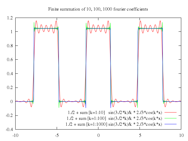
## data statistics
[Original Demo](http://gnuplot.sourceforge.net/demo_4.6/stats.html)
### 1
```ruby
# # Exercise the "stats" command.
# # Skip this demo cleanly if the stats option was not configured.
# #
# if (!strstrt(GPVAL_COMPILE_OPTIONS,"+STATS")) {
# print "No support for stats command"
# } else {
#
# set title "Use of stats command to find min/max/mean before plotting\nOne data column"
#
# set style data line
# set offset 0,0,.5,.5
# set autoscale fix
# set key left Left
#
# stats 'orbital_elements.dat' index 1 using 2 prefix "A"
#
# set arrow 1 from A_index_min, graph 0.1 to A_index_min, A_min fill
# set arrow 2 from A_index_max, graph 0.9 to A_index_max, A_max fill
# set label 1 "min" at A_index_min, graph 0.1 center offset 0,-1
# set label 2 "max" at A_index_max, graph 0.9 center offset 0,1
#
# plot 'orbital_elements.dat' index 1 using 0:2 title " Data" lw 2, \
# A_mean title " Mean"
Numo.gnuplot do
set title:"Use of stats command to find min/max/mean before plotting\nOne data column"
set :style, :data, :line
set offset:[0,0,0.5,0.5]
set autoscale:"fix"
set :key, :left, :Left
stats 'orbital_elements.dat', index:1, using:2, prefix:"A"
set :arrow, 1, from:"A_index_min, graph 0.1", to:"A_index_min, A_min", fill:true
set :arrow, 2, from:"A_index_max, graph 0.9", to:"A_index_max, A_max", fill:true
set :label, 1, "min", at:"A_index_min, graph 0.1", center:true, offset:[0,-1]
set :label, 2, "max", at:"A_index_max, graph 0.9", center:true, offset:[0,1]
plot ["'orbital_elements.dat'", index:1, using:[0,2], title:" Data", lw:2],
["A_mean", title:" Mean"]
end
```
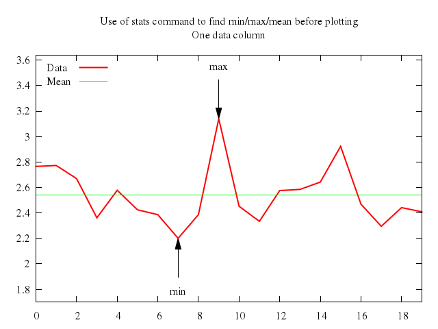
### 2
```ruby
# set title "Use of stats command to find min/max/mean before plotting\nTwo data columns"
#
# f(x) = log(1+x)
#
# stats 'orbital_elements.dat' index 1 using (f($0)):2 prefix "B"
#
# set arrow 1 from B_pos_min_y, graph 0.1 to B_pos_min_y, B_min_y fill
# set arrow 2 from B_pos_max_y, graph 0.9 to B_pos_max_y, B_max_y fill
# set label 1 "min" at B_pos_min_y, graph 0.1 center offset 0,-1
# set label 2 "max" at B_pos_max_y, graph 0.9 center offset 0,1
#
# plot 'orbital_elements.dat' index 1 using (f($0)):2 title " Data" lw 2, \
# B_mean_y title " Mean", \
# B_slope * x + B_intercept title "Linear fit"
Numo.gnuplot do
set title:"Use of stats command to find min/max/mean before plotting\nTwo data columns"
run "f(x) = log(1+x)"
stats 'orbital_elements.dat', index:1, using:'(f($0)):2', prefix:"B"
set :arrow, 1, from:"B_pos_min_y, graph 0.1", to:"B_pos_min_y, B_min_y", fill:true
set :arrow, 2, from:"B_pos_max_y, graph 0.9", to:"B_pos_max_y, B_max_y", fill:true
set :label, 1, "min", at:"B_pos_min_y, graph 0.1", center:true, offset:[0,-1]
set :label, 2, "max", at:"B_pos_max_y, graph 0.9", center:true, offset:[0,1]
plot ["'orbital_elements.dat'", index:1, using:'(f($0)):2', title:" Data", lw:2],
["B_mean_y", title:" Mean"],
["B_slope *", 'x+B_intercept', title:"Linear fit"]
end
```
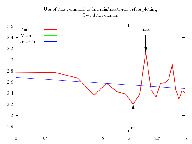
## surfaces 1
[Original Demo](http://gnuplot.sourceforge.net/demo_4.6/surface1.html)
### 1
```ruby
# set samples 21
# set isosample 11
# set xlabel "X axis" offset -3,-2
# set ylabel "Y axis" offset 3,-2
# set zlabel "Z axis" offset -5
# set title "3D gnuplot demo"
# set label 1 "This is the surface boundary" at -10,-5,150 center
# set arrow 1 from -10,-5,120 to -10,0,0 nohead
# set arrow 2 from -10,-5,120 to 10,0,0 nohead
# set arrow 3 from -10,-5,120 to 0,10,0 nohead
# set arrow 4 from -10,-5,120 to 0,-10,0 nohead
# set xrange [-10:10]
# set yrange [-10:10]
# splot x*y
Numo.gnuplot do
set samples:21
set isosample:11
set xlabel:"X axis", offset:[-3,-2]
set ylabel:"Y axis", offset:[3,-2]
set zlabel:"Z axis", offset:-5
set title:"3D gnuplot demo"
set :label, 1, "This is the surface boundary", at:[-10,-5,150], center:true
set :arrow, 1, from:[-10,-5,120], to:[-10,0,0], nohead:true
set :arrow, 2, from:[-10,-5,120], to:[10,0,0], nohead:true
set :arrow, 3, from:[-10,-5,120], to:[0,10,0], nohead:true
set :arrow, 4, from:[-10,-5,120], to:[0,-10,0], nohead:true
set xrange:-10..10
set yrange:-10..10
splot "x*y"
end
```
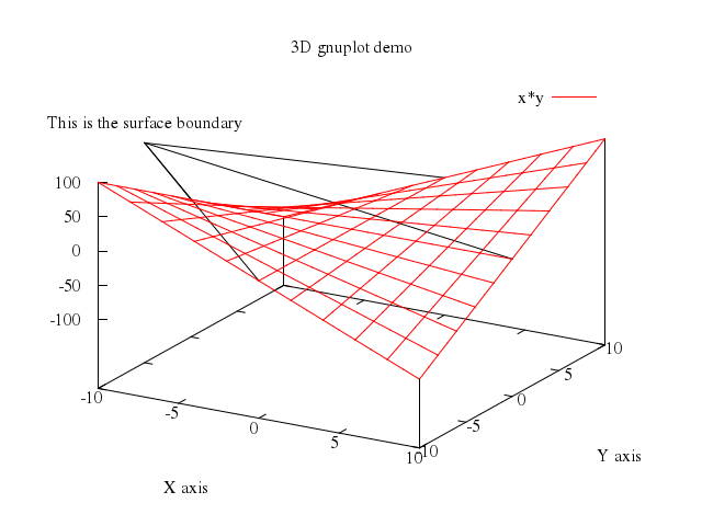
### 2
```ruby
# unset arrow
# unset label
# set grid
# splot x**2+y**2, x**2-y**2
Numo.gnuplot do
unset :arrow
unset :label
set :grid
splot "x**2+y**2",
"x**2-y**2"
end
```
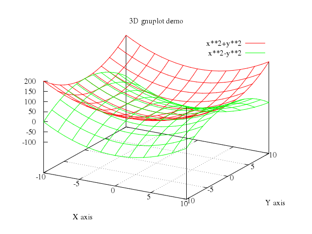
### 3
```ruby
# rep x*y
Numo.gnuplot do
replot "x*y"
end
```
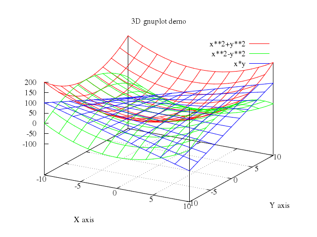
### 4
```ruby
# rep (x**3+y**3)/10
Numo.gnuplot do
replot "(x**3+y**3)/10"
end
```

### 5
```ruby
# set ticslevel 0.0
# set title "3D gnuplot demo ( ticslevel = 0.0 )"
# rep
Numo.gnuplot do
set ticslevel:0.0
set title:"3D gnuplot demo ( ticslevel = 0.0 )"
replot
end
```
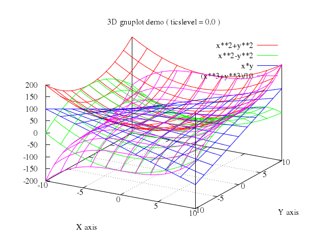
### 6
```ruby
# set ticslevel 2.0
# set title "3D gnuplot demo ( ticslevel = 2.0 )"
# rep
Numo.gnuplot do
set ticslevel:2.0
set title:"3D gnuplot demo ( ticslevel = 2.0 )"
replot
end
```
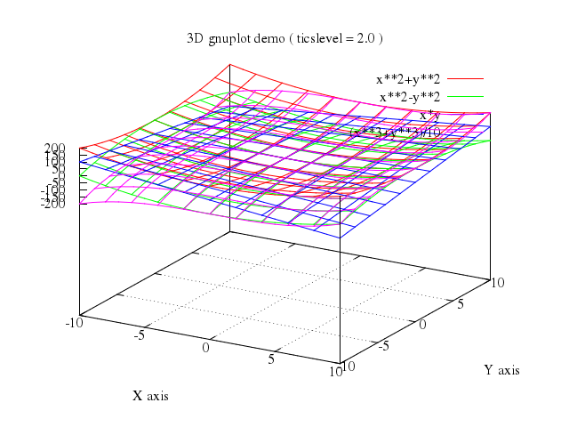
### 7
```ruby
# set ticslevel 0.5
# set title "3D gnuplot demo ( ticslevel = 0.5 )"
# rep
Numo.gnuplot do
set ticslevel:0.5
set title:"3D gnuplot demo ( ticslevel = 0.5 )"
replot
end
```
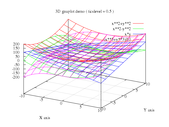
### 8
```ruby
# set title "3D gnuplot demo"
# unset grid
# splot x*y with points
Numo.gnuplot do
set title:"3D gnuplot demo"
unset :grid
splot "x*y", with:"points"
end
```
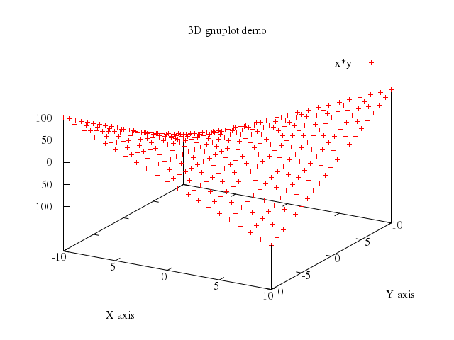
### 9
```ruby
# unset xtics
# unset ytics
# set xrange [-1:1]
# set yrange [-1:1]
# set title "Surfaces with no grid or tics"
# splot x*y with lines, x**2*y**3 with dots, x**3*y*2 with points
Numo.gnuplot do
unset :xtics
unset :ytics
set xrange:-1..1
set yrange:-1..1
set title:"Surfaces with no grid or tics"
splot ["x*y", with:"lines"],
["x**2*y**3", with:"dots"],
["x**3*y*2", with:"points"]
end
```
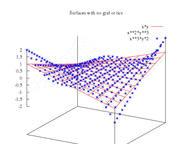
### 10
```ruby
# set xtics ("low" -3, "mid" 0, "high" 3)
# set ytics -2,0.5,2
# set xrange [-3:3]
# set yrange [-3:3]
# set log z
# set title "Surfaces with z log scale"
# splot x**2*y**2 + 2, x**2*y**4 + 2, x**4*y**2 + 2
Numo.gnuplot do
set xtics:'("low" -3, "mid" 0, "high" 3)'
set ytics:[-2,0.5,2]
set xrange:-3..3
set yrange:-3..3
set log:"z"
set title:"Surfaces with z log scale"
splot "x**2*y**2 + 2",
"x**2*y**4 + 2",
"x**4*y**2 + 2"
end
```
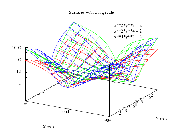
### 11
```ruby
# unset log z
# set xtics autofreq
# set ytics autofreq
# set xrange [-1:1]
# set yrange [-1:1]
# set samples 51
# set isosample 21
# set dummy u,v
# set title "3D gnuplot demo"
# splot u*v / (u**2 + v**2 + 0.1)
Numo.gnuplot do
unset log:"z"
set xtics:"autofreq"
set ytics:"autofreq"
set xrange:-1..1
set yrange:-1..1
set samples:51
set isosample:21
set dummy:"u,v"
set title:"3D gnuplot demo"
splot "u*v / (u**2 + v**2 + 0.1)"
end
```
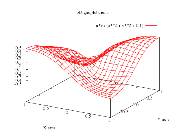
### 12
```ruby
# splot [x=-3:3] [y=-3:3] sin(x) * cos(y)
Numo.gnuplot do
splot "[x=-3:3]","[y=-3:3]",
"sin(x) * cos(y)"
end
```
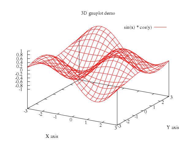
### 13
```ruby
# set zrange [-1.0:1.0]
# replot
Numo.gnuplot do
set zrange:-1.0..1.0
replot
end
```
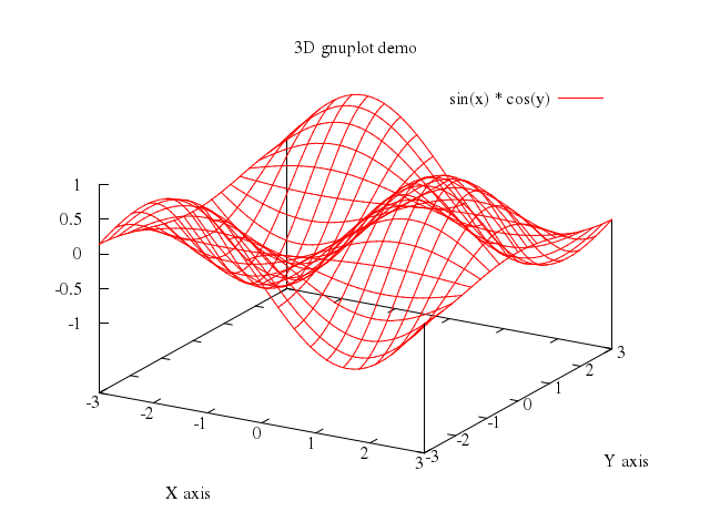
### 14
```ruby
# set title "Sinc function"
# set zrange [-1:1]
# set label 1 "This is equal to 1" at 0,3.2,1 left
# set arrow 1 from 0,3,1 to 0,0,1
# sinc(u,v) = sin(sqrt(u**2+v**2)) / sqrt(u**2+v**2)
# splot [-5:5.01] [-5:5.01] sinc(u,v)
Numo.gnuplot do
set title:"Sinc function"
set zrange:-1..1
set :label, 1, "This is equal to 1", at:[0,3.2,1], left:true
set :arrow, 1, from:[0,3,1], to:[0,0,1]
run "sinc(u,v) = sin(sqrt(u**2+v**2)) / sqrt(u**2+v**2)"
splot -5..5.01, -5..5.01,
"sinc(u,v)"
end
```
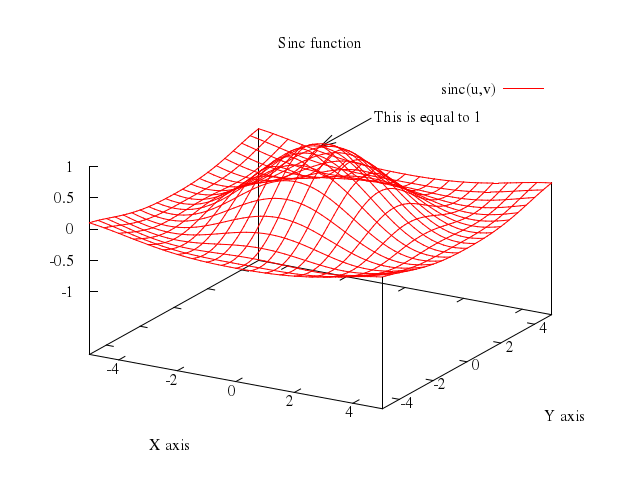
### 15
```ruby
# set view 70,20,1
# set zrange [-0.5:1.0]
# set ztics -1,0.25,1
# set label 1 "This is equal to 1" at -5,-2,1.5 centre
# set arrow 1 from -5,-2.1,1.4 to 0,0,1
# splot [-12:12.01] [-12:12.01] sinc(u,v)
Numo.gnuplot do
set view:[70,20,1]
set zrange:-0.5..1.0
set ztics:[-1,0.25,1]
set :label, 1, "This is equal to 1", at:[-5,-2,1.5], centre:true
set :arrow, 1, from:[-5,-2.1,1.4], to:[0,0,1]
splot -12..12.01, -12..12.01,
"sinc(u,v)"
end
```
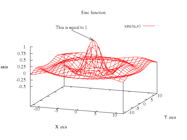
### 16
```ruby
# set title "\"fence plot\" using separate parametric surfaces"
# # A method suggested by Hans-Bernhard Broeker
# # : display a separate parametric
# # surface for each fence.
# set zrange [-1:1]
# unset label
# unset arrow
# set xrange [-5:5]; set yrange [-5:5]
# set arrow from 5,-5,-1.2 to 5,5,-1.2 lt -1
# set label 1 "increasing v" at 6,0,-1
# set arrow from 5,6,-1 to 5,5,-1 lt -1
# set label 2 "u=0" at 5,6.5,-1
# set arrow from 5,6,sinc(5,5) to 5,5,sinc(5,5) lt -1
# set label 3 "u=1" at 5,6.5,sinc(5,5)
# set parametric
# set hidden3d
# set isosamples 2,33
# xx=-5; dx=(4.99-(-4.99))/9
# x0=xx; xx=xx+dx
# x1=xx; xx=xx+dx
# x2=xx; xx=xx+dx
# x3=xx; xx=xx+dx
# x4=xx; xx=xx+dx
# x5=xx; xx=xx+dx
# x6=xx; xx=xx+dx
# x7=xx; xx=xx+dx
# x8=xx; xx=xx+dx
# x9=xx; xx=xx+dx
# splot [u=0:1][v=-4.99:4.99] \
# x0, v, (u<0.5) ? -1 : sinc(x0,v) notitle, \
# x1, v, (u<0.5) ? -1 : sinc(x1,v) notitle, \
# x2, v, (u<0.5) ? -1 : sinc(x2,v) notitle, \
# x3, v, (u<0.5) ? -1 : sinc(x3,v) notitle, \
# x4, v, (u<0.5) ? -1 : sinc(x4,v) notitle, \
# x5, v, (u<0.5) ? -1 : sinc(x5,v) notitle, \
# x6, v, (u<0.5) ? -1 : sinc(x6,v) notitle, \
# x7, v, (u<0.5) ? -1 : sinc(x7,v) notitle, \
# x8, v, (u<0.5) ? -1 : sinc(x8,v) notitle, \
# x9, v, (u<0.5) ? -1 : sinc(x9,v) notitle
Numo.gnuplot do
set title:"\"fence plot\" using separate parametric surfaces"
set zrange:-1..1
unset :label
unset :arrow
set xrange:-5..5; set yrange:-5..5
set :arrow, from:[5,-5,-1.2], to:[5,5,-1.2], lt:-1
set :label, 1, "increasing v", at:[6,0,-1]
set :arrow, from:[5,6,-1], to:[5,5,-1], lt:-1
set :label, 2, "u=0", at:[5,6.5,-1]
set :arrow, from:"5,6,sinc(5,5)", to:"5,5,sinc(5,5)", lt:-1
set :label, 3, "u=1", at:"5,6.5,sinc(5,5)"
set :parametric
set :hidden3d
set isosamples:[2,33]
run "xx=-5; dx=(4.99-(-4.99))/9"
run "x0=xx; xx=xx+dx"
run "x1=xx; xx=xx+dx"
run "x2=xx; xx=xx+dx"
run "x3=xx; xx=xx+dx"
run "x4=xx; xx=xx+dx"
run "x5=xx; xx=xx+dx"
run "x6=xx; xx=xx+dx"
run "x7=xx; xx=xx+dx"
run "x8=xx; xx=xx+dx"
run "x9=xx; xx=xx+dx"
splot "[u=0:1]","[v=-4.99:4.99]",
"x0",
"v",
["(u<0.5) ? -1 : sinc(x0,v)", :notitle],
"x1",
"v",
["(u<0.5) ? -1 : sinc(x1,v)", :notitle],
"x2",
"v",
["(u<0.5) ? -1 : sinc(x2,v)", :notitle],
"x3",
"v",
["(u<0.5) ? -1 : sinc(x3,v)", :notitle],
"x4",
"v",
["(u<0.5) ? -1 : sinc(x4,v)", :notitle],
"x5",
"v",
["(u<0.5) ? -1 : sinc(x5,v)", :notitle],
"x6",
"v",
["(u<0.5) ? -1 : sinc(x6,v)", :notitle],
"x7",
"v",
["(u<0.5) ? -1 : sinc(x7,v)", :notitle],
"x8",
"v",
["(u<0.5) ? -1 : sinc(x8,v)", :notitle],
"x9",
"v",
["(u<0.5) ? -1 : sinc(x9,v)", :notitle]
end
```
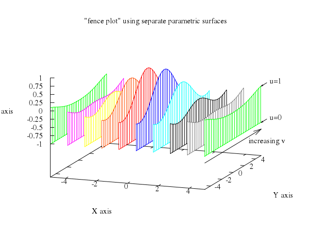
### 17
```ruby
# set title "\"fence plot\" using single parametric surface with undefined points"
# # Another method suggested by Hans-Bernhard Broeker
# # : Use parametric variable u to control
# # x, y, and z. u=3*fencenumber+remainder, where the remainder selects
# # one of three types of points:
# # remainder=0: x=xmin+fencenumber*dx, y=v, z=zbase
# # remainder=1: x=xmin+fencenumber*dx, y=v, z=f(x,y)
# # remainder=2: x=xmin+fencenumber*dx, y=v, z=1/0 (undefined)
# set parametric
# unset label
# unset arrow
# xmin=-4.99; xmax=5; n=10; dx=(xmax-xmin)/(n-1.)
# set isosamples 3*n,33
# zbase=-1
# set arrow from 5,-5,-1.2 to 5,5,-1.2 lt -1
# set label 1 "increasing v" at 6,0,-1
# set arrow from -5,-5,-1.2 to 5,-5,-1.2 lt -1
# set label 2 "increasing u" at 0,-5,-1.5
# set arrow from 5,6,-1 to 5,5,-1 lt -1
# set label 3 "floor(u)%3=0" at 5,6.5,-1
# set arrow from 5,6,sinc(5,5) to 5,5,sinc(5,5) lt -1
# set label 4 "floor(u)%3=1" at 5,6.5,sinc(5,5)
# splot [u=.5:3*n-.5][v=-4.99:4.99] \
# xmin+floor(u/3)*dx, v, ((floor(u)%3)==0) ? zbase : \
# (((floor(u)%3)==1) ? sinc(xmin+u/3.*dx,v) : 1/0) notitle
Numo.gnuplot do
set title:"\"fence plot\" using single parametric surface with undefined points"
set :parametric
unset :label
unset :arrow
run "xmin=-4.99; xmax=5; n=10; dx=(xmax-xmin)/(n-1.)"
set isosamples:'3*n,33'
run "zbase=-1"
set :arrow, from:[5,-5,-1.2], to:[5,5,-1.2], lt:-1
set :label, 1, "increasing v", at:[6,0,-1]
set :arrow, from:[-5,-5,-1.2], to:[5,-5,-1.2], lt:-1
set :label, 2, "increasing u", at:[0,-5,-1.5]
set :arrow, from:[5,6,-1], to:[5,5,-1], lt:-1
set :label, 3, "floor(u)%3=0", at:[5,6.5,-1]
set :arrow, from:"5,6,sinc(5,5)", to:"5,5,sinc(5,5)", lt:-1
set :label, 4, "floor(u)%3=1", at:"5,6.5,sinc(5,5)"
splot "[u=.5:3*n-.5]","[v=-4.99:4.99]",
"xmin+floor(u/3)*dx",
"v",
["((floor(u)%3)==0) ? zbase : (((floor(u)%3)==1) ? sinc(xmin+u/3.*dx,v) : 1/0)", :notitle]
end
```
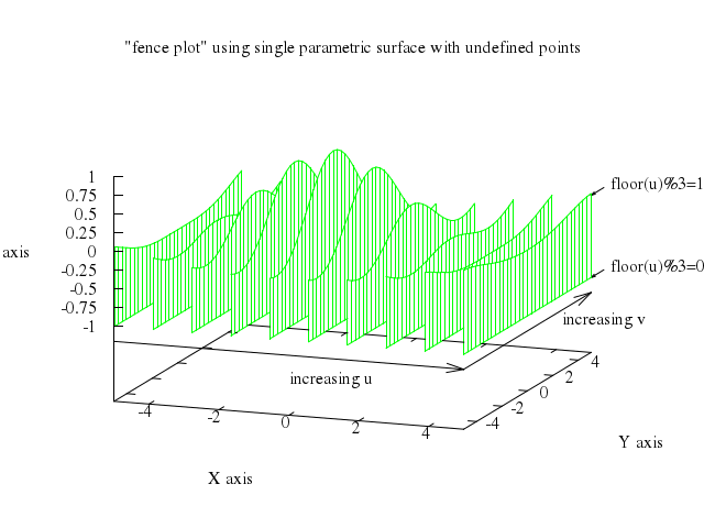
### 18
```ruby
# unset hidden3d; unset parametric; set isosamples 20,20
# set xrange [-1:1]; set yrange [-1:1]
# set ztics autofreq
# unset arrow
# unset label
# set log
# set auto
# set title "This has logarithmic scale"
# splot [x=1:15] [y=1:15] x**2+y**2
Numo.gnuplot do
unset :hidden3d; unset :parametric; set isosamples:[20,20]
set xrange:-1..1; set yrange:-1..1
set ztics:"autofreq"
unset :arrow
unset :label
set :log
set :auto
set title:"This has logarithmic scale"
splot "[x=1:15]","[y=1:15]",
"x**2+y**2"
end
```
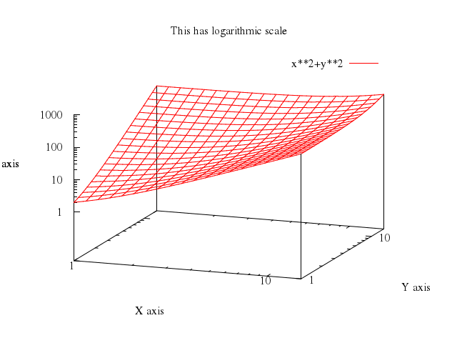
### 19
```ruby
# unset log
# set xrange [0:15]
# set yrange [0:15]
# set auto
# #set zrange [-0.6:0.7]
# set ticslevel 0
# set style data lines
# set title "Data grid plotting"
# set parametric
# splot "glass.dat"
Numo.gnuplot do
unset :log
set xrange:0..15
set yrange:0..15
set :auto
set ticslevel:0
set :style, :data, :lines
set title:"Data grid plotting"
set :parametric
splot "\"glass.dat\""
end
```
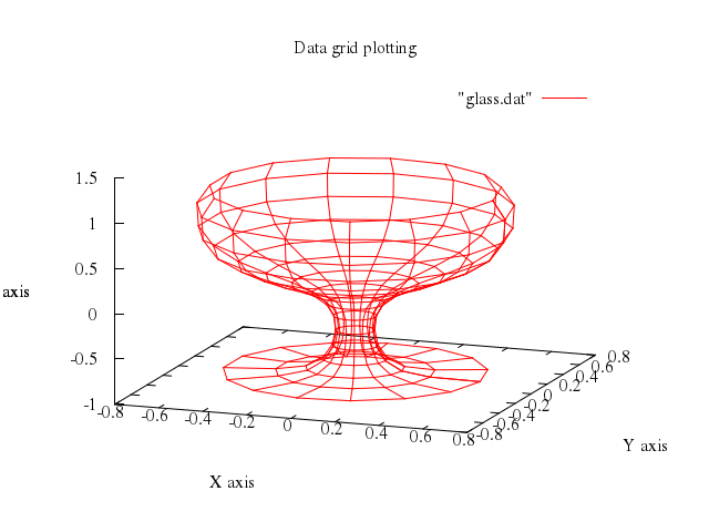
### 20
```ruby
# splot "glass.dat" using 3:2:1
Numo.gnuplot do
splot "\"glass.dat\"", using:[3,2,1]
end
```
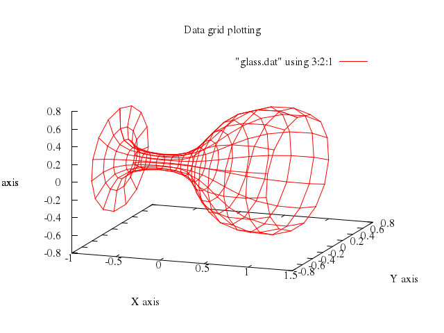
### 21
```ruby
# set zrange [-1.2:1.2]
# set ticslevel 0.5
# unset parametric
# set xlabel "line index within group"
# set ylabel "group index"
# splot "glass.dat" using 1, "glass.dat" using 2, "glass.dat" using 3
Numo.gnuplot do
set zrange:-1.2..1.2
set ticslevel:0.5
unset :parametric
set xlabel:"line index within group"
set ylabel:"group index"
splot ["\"glass.dat\"", using:1],
["\"glass.dat\"", using:2],
["\"glass.dat\"", using:3]
end
```
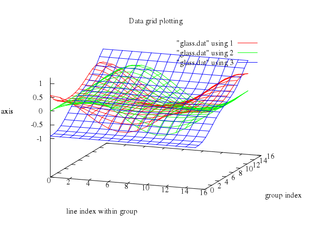
### 22
```ruby
# set title "splot of part of a data file"
# set xlabel "X axis" offset -3,-2
# set ylabel "Y axis" offset 3,-2
# set hidden3d
# splot 'glass.dat' every 2::0::12 with lines
Numo.gnuplot do
set title:"splot of part of a data file"
set xlabel:"X axis", offset:[-3,-2]
set ylabel:"Y axis", offset:[3,-2]
set :hidden3d
splot "'glass.dat'", every:"2::0::12", with:"lines"
end
```
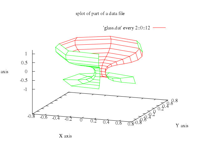
### 23
```ruby
# set title "splot with \"set pm3d\" (implemented with some terminals)"
# set pm3d
# set hidden3d
# splot 'glass.dat' every 2::0::12 with lines
Numo.gnuplot do
set title:"splot with \"set pm3d\" (implemented with some terminals)"
set :pm3d
set :hidden3d
splot "'glass.dat'", every:"2::0::12", with:"lines"
end
```
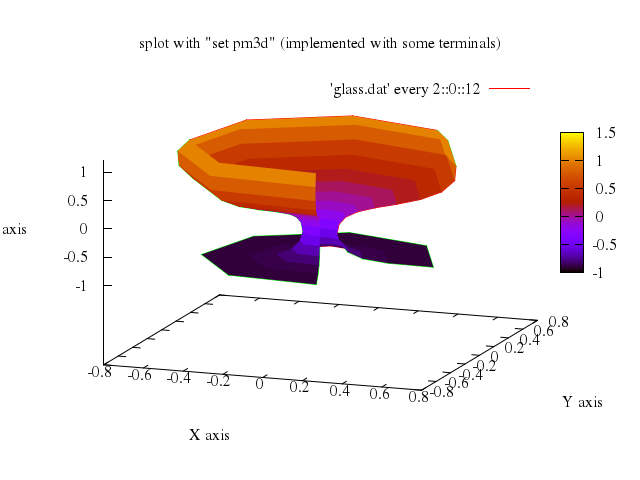
### 24
```ruby
# unset hidden3d
# unset pm3d
# set param
# set title "Test of spherical coordinates"
# set mapping spherical
# splot "glass.dat"
Numo.gnuplot do
unset :hidden3d
unset :pm3d
set :param
set title:"Test of spherical coordinates"
set mapping:"spherical"
splot "\"glass.dat\""
end
```
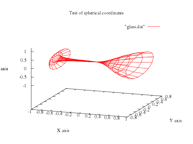
### 25
```ruby
# # mandelbrot demo
# set title "Mandelbrot function"
# unset parametric
# set mapping cartesian
# set view 60,30,1,1
# set auto
# set isosamples 60
# set hidden3d
# compl(a,b)=a*{1,0}+b*{0,1}
# mand(z,a,n) = n<=0 || abs(z)>100 ? 1:mand(z*z+a,a,n-1)+1
# splot [-2:1][-1.5:1.5] mand({0,0},compl(x,y),30)
Numo.gnuplot do
set title:"Mandelbrot function"
unset :parametric
set mapping:"cartesian"
set view:[60,30,1,1]
set :auto
set isosamples:60
set :hidden3d
run "compl(a,b)=a*{1,0}+b*{0,1}"
run "mand(z,a,n) = n<=0 || abs(z)>100 ? 1:mand(z*z+a,a,n-1)+1"
splot -2..1, -1.5..1.5,
"mand({0,0},compl(x,y),30)"
end
```
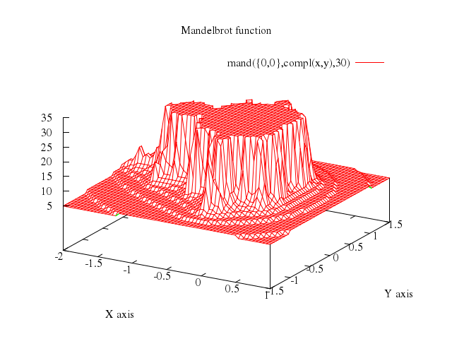
## surfaces 2
[Original Demo](http://gnuplot.sourceforge.net/demo_4.6/surface2.html)
### 1
```ruby
# set parametric
# set isosamples 50,10
# set hidden
# set key below
#
# set title "Parametric Sphere"
# set urange [-pi/2:pi/2]
# set vrange [0:2*pi]
# set ztics nomirror -1.0,0.25,1.0
# set view 45,50
# splot cos(u)*cos(v),cos(u)*sin(v),sin(u)
Numo.gnuplot do
set :parametric
set isosamples:[50,10]
set :hidden
set :key, "below"
set title:"Parametric Sphere"
set urange:"[-pi/2:pi/2]"
set vrange:"[0:2*pi]"
set :ztics, :nomirror, [-1.0,0.25,1.0]
set view:[45,50]
splot "cos(u)*cos(v)",
"cos(u)*sin(v)",
"sin(u)"
end
```
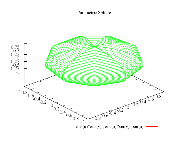
### 2
```ruby
# set view ,,,0.7
# set title "Parametric Sphere, crunched z axis"
# replot
Numo.gnuplot do
set view:',,,0.7'
set title:"Parametric Sphere, crunched z axis"
replot
end
```
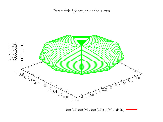
### 3
```ruby
# set view ,,,1.4
# set title "Parametric Sphere, enlarged z axis"
# replot
Numo.gnuplot do
set view:',,,1.4'
set title:"Parametric Sphere, enlarged z axis"
replot
end
```
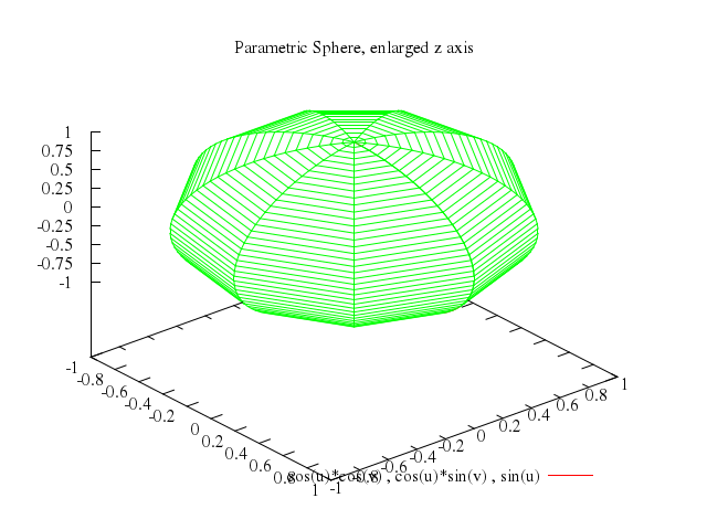
### 4
```ruby
# set view ,,,1.0
#
# set title "Parametric Torus"
# set urange [0:2*pi]
# set vrange [0:2*pi]
# set zrange [-1:1] # imitate old 'set view' hack
# splot (1-0.2*cos(v))*cos(u),(1-0.2*cos(v))*sin(u),0.2*sin(v)
Numo.gnuplot do
set view:',,,1.0'
set title:"Parametric Torus"
set urange:"[0:2*pi]"
set vrange:"[0:2*pi]"
set zrange:-1..1 # imitate old 'set view' hack
splot "(1-0.2*cos(v))*cos(u)",
"(1-0.2*cos(v))*sin(u)",
"0.2*sin(v)"
end
```
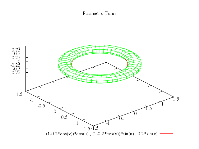
### 5
```ruby
# set title "Parametric Hexagon"
# set urange [-1.3:1.3]
# set vrange [0:2*pi]
# set autoscale z
# set ticslevel 0. # reserve more space z direction.
# set view ,,0.7,1.4 # crunch xyz, and re-extend z back to full size
# set ztics autofreq
# splot cos(v)**3*cos(u)**3,sin(v)**3*cos(u)**3,sin(u)**3
Numo.gnuplot do
set title:"Parametric Hexagon"
set urange:-1.3..1.3
set vrange:"[0:2*pi]"
set autoscale:"z"
set ticslevel:0.0 # reserve more space z direction.
set view:',,0.7,1.4' # crunch xyz, and re-extend z back to "full" size
set ztics:"autofreq"
splot "cos(v)**3*cos(u)**3",
"sin(v)**3*cos(u)**3",
"sin(u)**3"
end
```
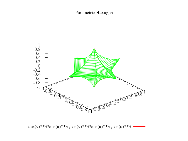
### 6
```ruby
# set view ,,1.,1.
#
# set title "Parametric Helix"
# set isosamples 100,20
# set urange [0:10*pi]
# set vrange [0:2*pi]
# set autoscale z
# splot (1-0.1*cos(v))*cos(u),(1-0.1*cos(v))*sin(u),0.1*(sin(v)+u/1.7-10)
Numo.gnuplot do
set view:',,1.,1.'
set title:"Parametric Helix"
set isosamples:[100,20]
set urange:"[0:10*pi]"
set vrange:"[0:2*pi]"
set autoscale:"z"
splot "(1-0.1*cos(v))*cos(u)",
"(1-0.1*cos(v))*sin(u)",
"0.1*(sin(v)+u/1.7-10)"
end
```
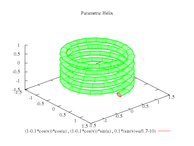
### 7
```ruby
# set title "Parametric Shell (clipped to limited z range)"
# set isosamples 40,20
# set view 50,30,1.0
# set urange [0:2*pi]
# set vrange [0:2*pi]
# set zrange [-3:1.5]
# splot cos(u)*u*(1+cos(v)/2),sin(v)*u/2,sin(u)*u*(1+cos(v)/2)
Numo.gnuplot do
set title:"Parametric Shell (clipped to limited z range)"
set isosamples:[40,20]
set view:[50,30,1.0]
set urange:"[0:2*pi]"
set vrange:"[0:2*pi]"
set zrange:-3..1.5
splot "cos(u)*u*(1+cos(v)/2)",
"sin(v)*u/2",
"sin(u)*u*(1+cos(v)/2)"
end
```
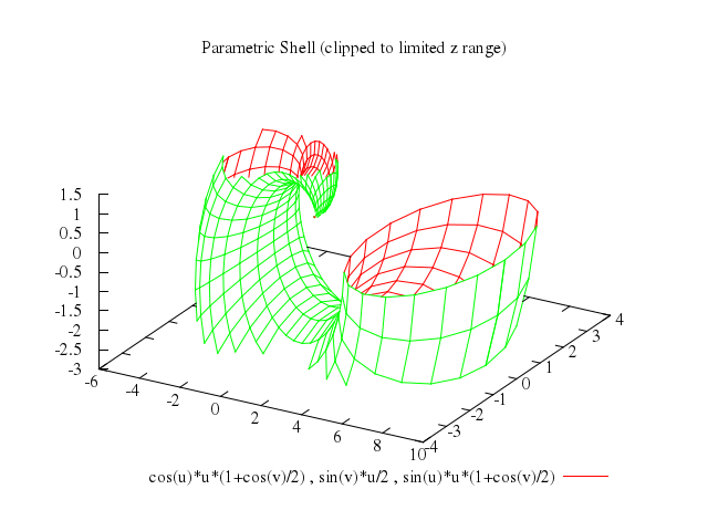
### 8
```ruby
# set autoscale z
# set title "Parametric Shell (automatic z range)"
# replot
Numo.gnuplot do
set autoscale:"z"
set title:"Parametric Shell (automatic z range)"
replot
end
```
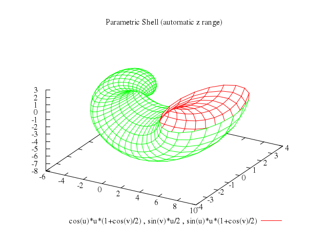
### 9
```ruby
# set title "Interlocking Tori"
#
# set urange [-pi:pi]
# set vrange [-pi:pi]
# set isosamples 50,20
# splot cos(u)+.5*cos(u)*cos(v),sin(u)+.5*sin(u)*cos(v),.5*sin(v) with lines, \
# 1+cos(u)+.5*cos(u)*cos(v),.5*sin(v),sin(u)+.5*sin(u)*cos(v) with lines
Numo.gnuplot do
set title:"Interlocking Tori"
set urange:"[-pi:pi]"
set vrange:"[-pi:pi]"
set isosamples:[50,20]
splot "cos(u)+.5*cos(u)*cos(v)",
"sin(u)+.5*sin(u)*cos(v)",
[".5*sin(v)", with:"lines"],
"1+cos(u)+.5*cos(u)*cos(v)",
".5*sin(v)",
["sin(u)+.5*sin(u)*cos(v)", with:"lines"]
end
```
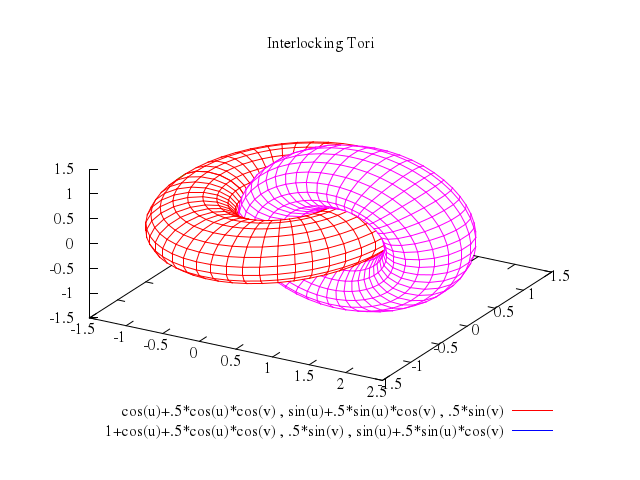
## contours
[Original Demo](http://gnuplot.sourceforge.net/demo_4.6/contours.html)
### 1
```ruby
# set samples 20
# set isosamples 21
# set xlabel "X axis"
# set ylabel "Y axis"
# set zlabel "Z axis" offset 1, 0
# set view 60, 30, 0.85, 1.1
# set title "3D gnuplot demo - contour plot"
# set contour
# splot x*y
Numo.gnuplot do
set samples:20
set isosamples:21
set xlabel:"X axis"
set ylabel:"Y axis"
set zlabel:"Z axis", offset:[1,0]
set view:[60,30,0.85,1.1]
set title:"3D gnuplot demo - contour plot"
set :contour
splot "x*y"
end
```
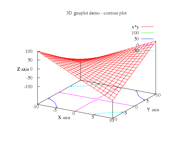
### 2
```ruby
# set cntrparam levels 20
# set title "3D gnuplot demo - contour plot (more contours)"
# replot
Numo.gnuplot do
set :cntrparam, levels:20
set title:"3D gnuplot demo - contour plot (more contours)"
replot
end
```
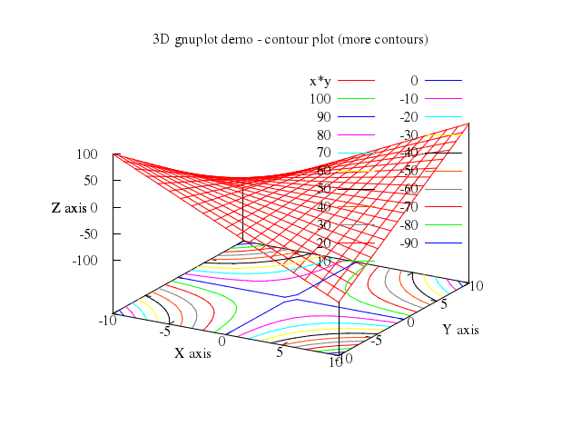
### 3
```ruby
# set cntrparam levels incr -100,10,100
# set title "3D gnuplot demo - contour plot (every 10, starting at -100)"
# replot
Numo.gnuplot do
set :cntrparam, :levels, incr:[-100,10,100]
set title:"3D gnuplot demo - contour plot (every 10, starting at -100)"
replot
end
```
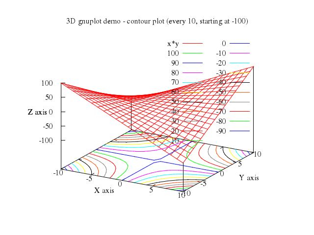
### 4
```ruby
# set cntrparam levels disc -75,-50,0
# set title "3D gnuplot demo - contour plot (at -75, -50, 0)"
# replot
Numo.gnuplot do
set :cntrparam, :levels, disc:[-75,-50,0]
set title:"3D gnuplot demo - contour plot (at -75, -50, 0)"
replot
end
```
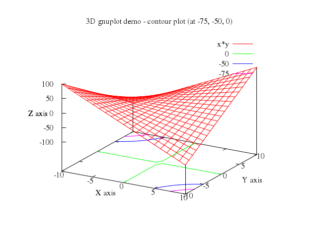
### 5
```ruby
# set cntrparam levels auto 10
# set title "3D gnuplot demo - contour plot on base grid"
# set contour base
# splot x**2-y**2
Numo.gnuplot do
set :cntrparam, :levels, auto:10
set title:"3D gnuplot demo - contour plot on base grid"
set contour:"base"
splot "x**2-y**2"
end
```
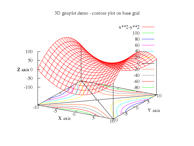
### 6
```ruby
# set title "3D gnuplot demo - contour plot on surface"
# set contour surface
# replot
Numo.gnuplot do
set title:"3D gnuplot demo - contour plot on surface"
set :contour, :surface
replot
end
```
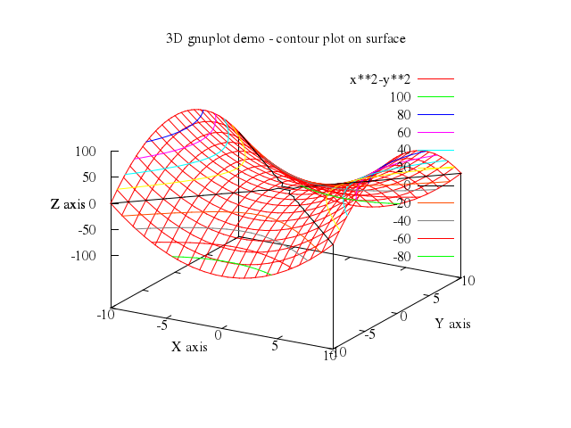
### 7
```ruby
# set title "3D gnuplot demo - contour plot on both"
# set contour both
# replot
Numo.gnuplot do
set title:"3D gnuplot demo - contour plot on both"
set contour:"both"
replot
end
```
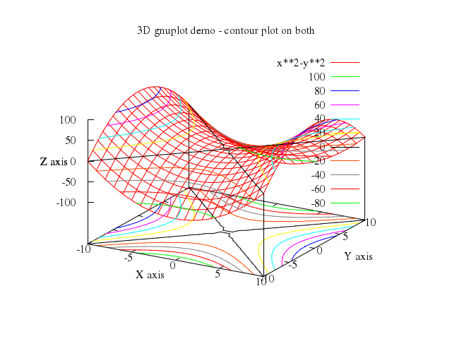
### 8
```ruby
# set contour base
# set title "3D gnuplot demo - 2 surfaces"
# splot x**2*y**3, x**3*y**2
Numo.gnuplot do
set contour:"base"
set title:"3D gnuplot demo - 2 surfaces"
splot "x**2*y**3",
"x**3*y**2"
end
```
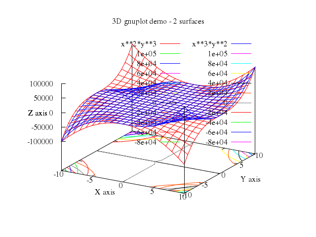
### 9
```ruby
# set title "3D gnuplot demo - some more interesting contours"
# splot x*y / (x**2 + y**2 + 0.1)
Numo.gnuplot do
set title:"3D gnuplot demo - some more interesting contours"
splot "x*y / (x**2 + y**2 + 0.1)"
end
```
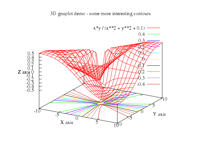
### 10
```ruby
# splot [x=-3:3] [y=-3:3] sin(x) * cos(y)
Numo.gnuplot do
splot "[x=-3:3]","[y=-3:3]",
"sin(x) * cos(y)"
end
```
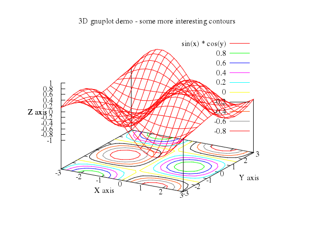
### 11
```ruby
# set zrange [-1.0:1.0]
# replot
Numo.gnuplot do
set zrange:-1.0..1.0
replot
end
```
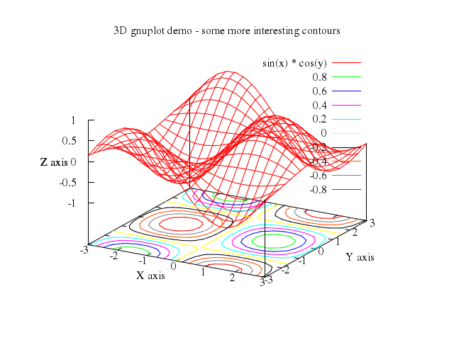
### 12
```ruby
# set samples 6
# set isosamples 6
# set cntrparam levels 5
# set title "3D gnuplot demo - low resolution (6x6)"
# replot
Numo.gnuplot do
set samples:6
set isosamples:6
set :cntrparam, levels:5
set title:"3D gnuplot demo - low resolution (6x6)"
replot
end
```
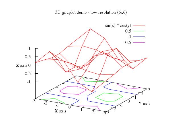
### 13
```ruby
# set cntrparam bspline
# set title "3D gnuplot demo - low resolution (6x6) using bspline approx."
# replot
Numo.gnuplot do
set :cntrparam, "bspline"
set title:"3D gnuplot demo - low resolution (6x6) using bspline approx."
replot
end
```
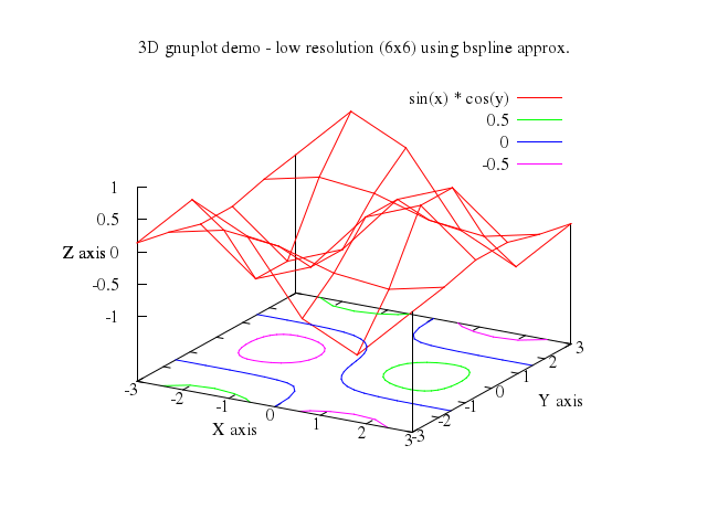
### 14
```ruby
# set cntrparam order 8
# set title "3D gnuplot demo - low resolution (6x6) raise bspline order."
# replot
Numo.gnuplot do
set :cntrparam, order:8
set title:"3D gnuplot demo - low resolution (6x6) raise bspline order."
replot
end
```

### 15
```ruby
# set cntrparam linear
# set auto
# set title "3D gnuplot demo - low resolution (6x6) using linear contours."
# splot x*y
Numo.gnuplot do
set :cntrparam, "linear"
set :auto
set title:"3D gnuplot demo - low resolution (6x6) using linear contours."
splot "x*y"
end
```
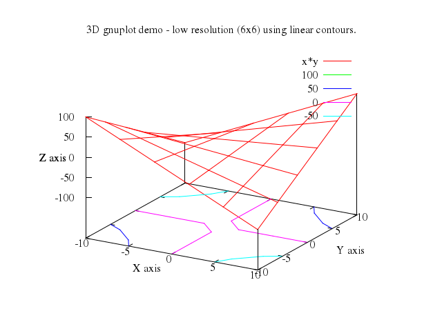
### 16
```ruby
# set cntrparam order 4
# set cntrparam bspline
# set title "3D gnuplot demo - low resolution (6x6) using bspline approx."
# replot
Numo.gnuplot do
set :cntrparam, order:4
set :cntrparam, "bspline"
set title:"3D gnuplot demo - low resolution (6x6) using bspline approx."
replot
end
```
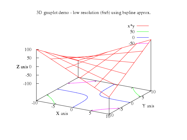
### 17
```ruby
# set samples 25
# set isosamples 26
# set title "3D gnuplot demo - contour of Sinc function"
# splot [-5:5.01] [-5:5.01] sin(sqrt(x**2+y**2)) / sqrt(x**2+y**2)
Numo.gnuplot do
set samples:25
set isosamples:26
set title:"3D gnuplot demo - contour of Sinc function"
splot -5..5.01, -5..5.01,
"sin(sqrt(x**2+y**2)) / sqrt(x**2+y**2)"
end
```
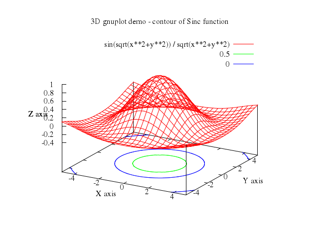
### 18
```ruby
# splot [-12:12.01] [-12:12.01] sin(sqrt(x**2+y**2)) / sqrt(x**2+y**2)
Numo.gnuplot do
splot -12..12.01, -12..12.01,
"sin(sqrt(x**2+y**2)) / sqrt(x**2+y**2)"
end
```
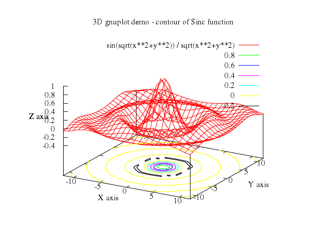
### 19
```ruby
# set cntrparam levels 10
# set auto
# set zrange [-1.0:1.0]
# set style data lines
# set title "3D gnuplot demo - contour of data grid plotting"
# set parametric
# splot "glass.dat"
Numo.gnuplot do
set :cntrparam, levels:10
set :auto
set zrange:-1.0..1.0
set :style, :data, :lines
set title:"3D gnuplot demo - contour of data grid plotting"
set :parametric
splot "\"glass.dat\""
end
```
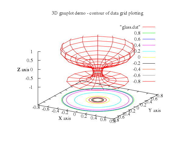
### 20
```ruby
# set xrange [0:15]
# set yrange [0:15]
# set zrange [-1.2:1.2]
# unset parametric
# splot "glass.dat" using 1
Numo.gnuplot do
set xrange:0..15
set yrange:0..15
set zrange:-1.2..1.2
unset :parametric
splot "\"glass.dat\"", using:1
end
```
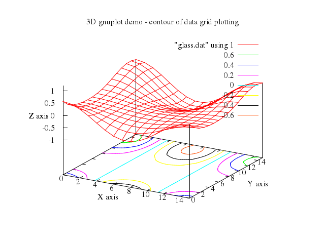
### 21
```ruby
# set view map
# unset surface
# set title "3D gnuplot demo - 2D contour projection of last plot"
# replot
Numo.gnuplot do
set view:'map'
unset :surface
set title:"3D gnuplot demo - 2D contour projection of last plot"
replot
end
```
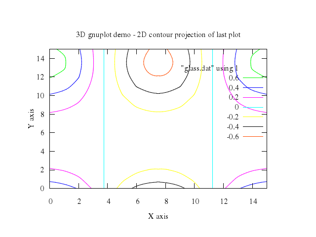
### 22
```ruby
# #From: [email protected] (Mingzuo Shen)
# #Subject: Rosenbrock's function: some answers and thanks
# #Date: Wed, 23 Jun 1993 20:50:36 GMT
# #
# # Last night I asked for help with a contour plot for the function:
# #
# # (1-x)**2 + 100 * (y - x**2)**2
# #
# #which should have a minimum at (x=1,y=1). This is the 2D case of a more
# #general function named after Rosenbrock (the book I am reading does not
# #give a reference to any paper/book by this person):
# #
# # for even integer n,
# #
# # f(x) = \sum_{j=1,3,5,\ldots,n} [(1 - x_j)^2 + 100(x_{j+1} - x_j^2)^2]
# #
# #where x is a vector (x1, x2, ..., x_n). This function also have a minimum
# #at (1,1,...,1), which lies at the base of a "banana-shaped valley".
# #Here are the new commands I have tried.
# #
# set auto
# set surface
# unset contour
# set cntrparam levels 5
# set cntrparam linear
# set samples 100
# set logscale z
# set hidden3d
# set isosamples 20
# set view 70,335,1,1
# set xlabel "x"
# set ylabel "y"
# set title "Rosenbrock Function"
# splot [0.9:1.1] [0.9:1.1] (1-x)**2 + 100*(y - x**2)**2
Numo.gnuplot do
set :auto
set :surface
unset :contour
set :cntrparam, levels:5
set :cntrparam, "linear"
set samples:100
set logscale:"z"
set :hidden3d
set isosamples:20
set view:[70,335,1,1]
set xlabel:"x"
set ylabel:"y"
set title:"Rosenbrock Function"
splot 0.9..1.1, 0.9..1.1,
"(1-x)**2 + 100*(y - x**2)**2"
end
```
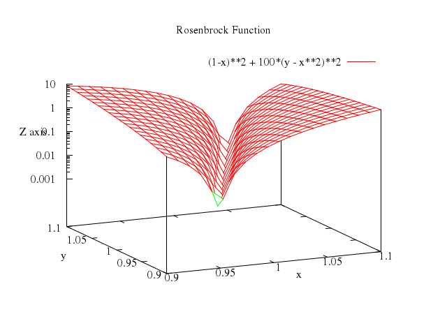
### 23
```ruby
# set logscale z
# set hidden3d
# set isosamples 60
# set ticslevel 0.
# set view 20,340 #HBB: ,1,2
# set xlabel "x"
# set ylabel "y"
# splot [-1.5:1.5] [-0.5:1.5] (1-x)**2 + 100*(y - x**2)**2
Numo.gnuplot do
set logscale:"z"
set :hidden3d
set isosamples:60
set ticslevel:0.0
set view:[20,340] #HBB: ,1,2
set xlabel:"x"
set ylabel:"y"
splot -1.5..1.5, -0.5..1.5,
"(1-x)**2 + 100*(y - x**2)**2"
end
```
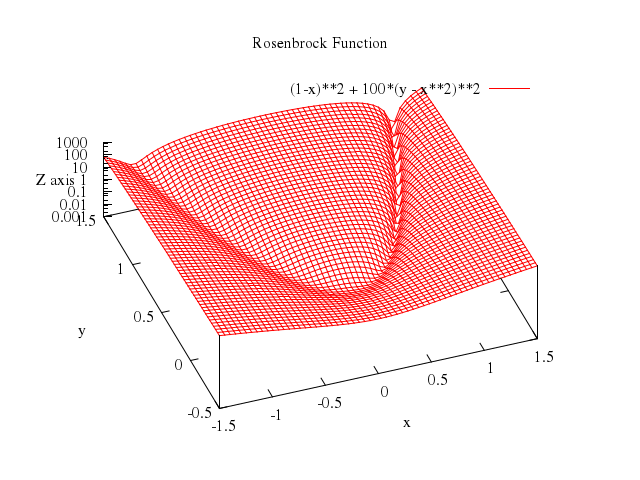
### 24
```ruby
# set contour
# unset surface
# unset ztics
# unset zlabel
# set border 15
# replot
Numo.gnuplot do
set :contour
unset :surface
unset :ztics
unset :zlabel
set border:15
replot
end
```
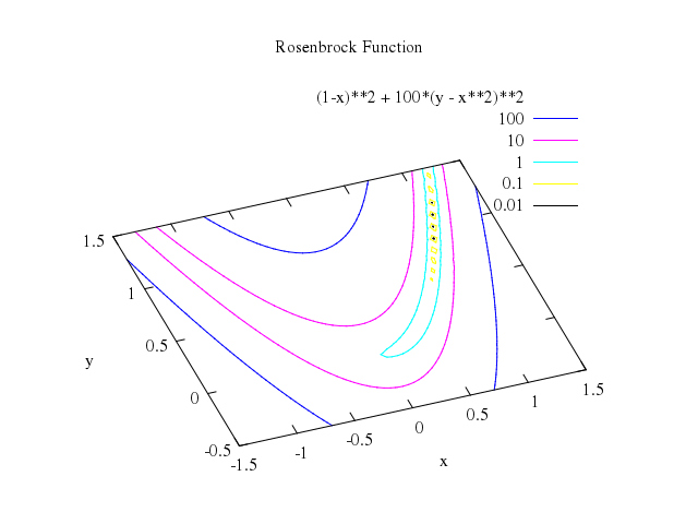
### 25
```ruby
# set title "All contours drawn in a single color"
# unset clabel
# splot [-1.5:1.5] [-0.5:1.5] (1-x)**2 + 100*(y - x**2)**2 with lines lc rgb "#007700"
Numo.gnuplot do
set title:"All contours drawn in a single color"
unset :clabel
splot -1.5..1.5, -0.5..1.5,
"(1-x)**2 + 100*(y - x**2)**2", with:"lines", lc_rgb:"#007700"
end
```
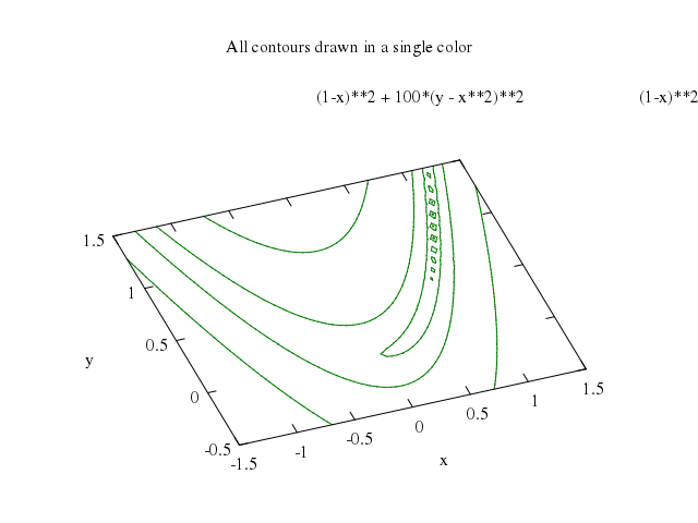
## singularities
[Original Demo](http://gnuplot.sourceforge.net/demo_4.6/singulr.html)
### 1
```ruby
# # $Id: singulr.dem,v 1.6 2003/10/28 05:35:54 sfeam Exp $
# #
# # Demo that plots some surfaces with singularities.
# # Author: Carsten Steger
# #
# # (x,y,x^2-y^2,2xy) is the graph of w=z^2 in 4-space.
# # Therefore (x^2-y^2,2xy,x,y) is the graph of w=sqrt(z) in 4-space.
# # Coordinates 1, 2, and 3 give the real part of either function,
# # whereas coordinates 1, 2, and 4 give the imaginary part.
# # The same holds for the cube function w=z^3. The graphs are given by
# # (x,y,x^3-3xy^2,3x^2y-y^3) and (x^3-3xy^2,3x^2y-y^3,x,y).
# # And so on...
#
# set parametric
# set hidden3d
# set isosamples 21
# set autoscale
#
# set view 60,30
# set urange [-3:3]
# set vrange [-3:3]
# set title "Real part of complex square root function"
# splot u**2-v**2,2*u*v,u
Numo.gnuplot do
set :parametric
set :hidden3d
set isosamples:21
set :autoscale
set view:[60,30]
set urange:-3..3
set vrange:-3..3
set title:"Real part of complex square root function"
splot "u**2-v**2",
"2*u*v",
"u"
end
```
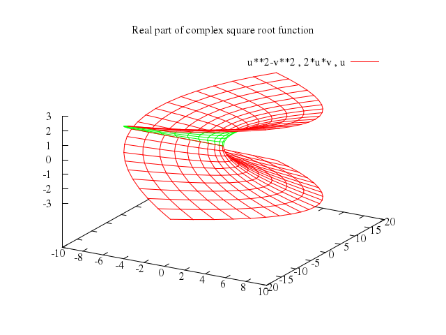
### 2
```ruby
# set view 60,210
# set title "Real part of complex square root function (different view)"
# replot
Numo.gnuplot do
set view:[60,210]
set title:"Real part of complex square root function (different view)"
replot
end
```
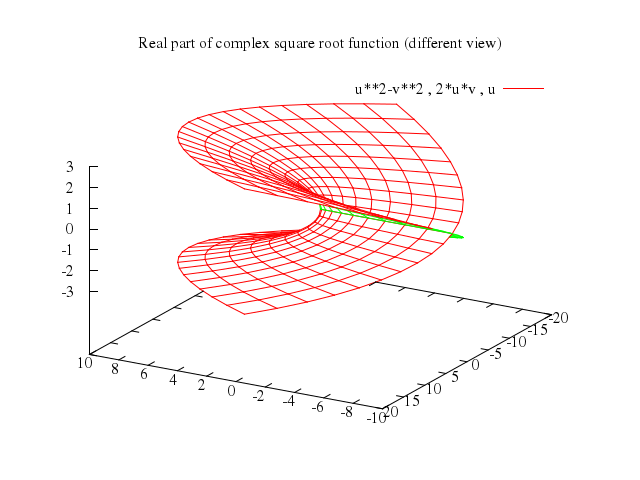
### 3
```ruby
# set view 60,120
# set urange [-3:3]
# set vrange [-3:3]
# set title "Imaginary part of complex square root function"
# splot u**2-v**2,2*u*v,v
Numo.gnuplot do
set view:[60,120]
set urange:-3..3
set vrange:-3..3
set title:"Imaginary part of complex square root function"
splot "u**2-v**2",
"2*u*v",
"v"
end
```
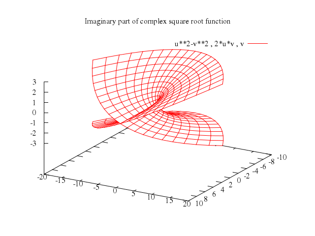
### 4
```ruby
# set view 60,300
# set title "Imaginary part of complex square root function (different view)"
# replot
Numo.gnuplot do
set view:[60,300]
set title:"Imaginary part of complex square root function (different view)"
replot
end
```
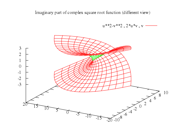
### 5
```ruby
# set view 60,30
# set urange [-3:3]
# set vrange [-3:3]
# set title "Real part of complex cube root function"
# splot u**3-3*u*v**2,3*u**2*v-v**3,u
Numo.gnuplot do
set view:[60,30]
set urange:-3..3
set vrange:-3..3
set title:"Real part of complex cube root function"
splot "u**3-3*u*v**2",
"3*u**2*v-v**3",
"u"
end
```
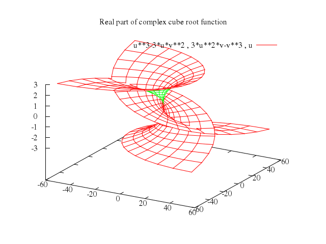
### 6
```ruby
# set view 60,210
# set title "Real part of complex cube root function (different view)"
# replot
Numo.gnuplot do
set view:[60,210]
set title:"Real part of complex cube root function (different view)"
replot
end
```
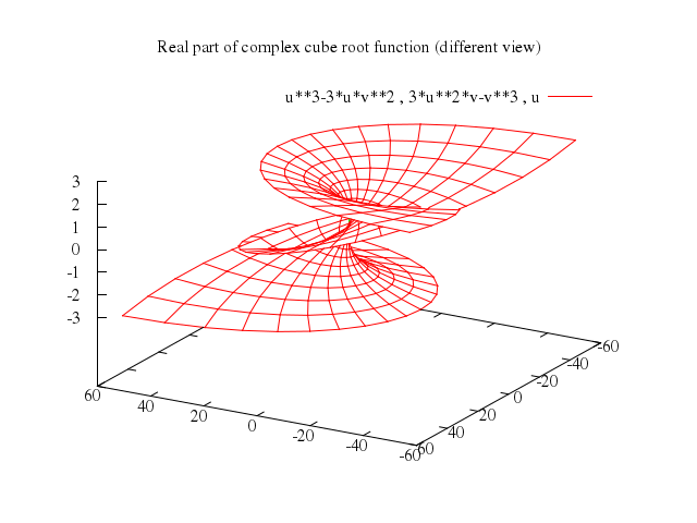
### 7
```ruby
# set view 60,30
# set urange [-3:3]
# set vrange [-3:3]
# set title "Imaginary part of complex cube root function"
# splot u**3-3*u*v**2,3*u**2*v-v**3,v
Numo.gnuplot do
set view:[60,30]
set urange:-3..3
set vrange:-3..3
set title:"Imaginary part of complex cube root function"
splot "u**3-3*u*v**2",
"3*u**2*v-v**3",
"v"
end
```
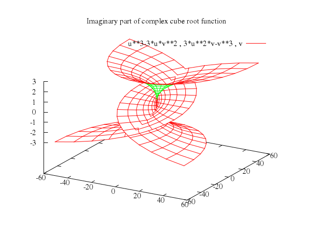
### 8
```ruby
# set view 60,210
# set title "Imaginary part of complex cube root function (different view)"
# replot
Numo.gnuplot do
set view:[60,210]
set title:"Imaginary part of complex cube root function (different view)"
replot
end
```
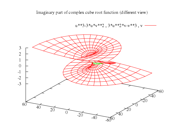
### 9
```ruby
# set view 60,30
# set isosamples 31
# set urange [-1:1]
# set vrange [-1:1]
# set title "Real part of complex 4th root function"
# splot u**4-6*u**2*v**2+v**4,4*u**3*v-4*u*v**3,u
Numo.gnuplot do
set view:[60,30]
set isosamples:31
set urange:-1..1
set vrange:-1..1
set title:"Real part of complex 4th root function"
splot "u**4-6*u**2*v**2+v**4",
"4*u**3*v-4*u*v**3",
"u"
end
```
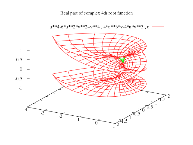
### 10
```ruby
# set view 60,210
# set title "Real part of complex 4th root function (different view)"
# replot
Numo.gnuplot do
set view:[60,210]
set title:"Real part of complex 4th root function (different view)"
replot
end
```
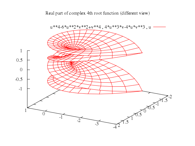
### 11
```ruby
# set view 60,120
# set urange [-1:1]
# set vrange [-1:1]
# set title "Imaginary part of complex 4th root function"
# splot u**4-6*u**2*v**2+v**4,4*u**3*v-4*u*v**3,v
Numo.gnuplot do
set view:[60,120]
set urange:-1..1
set vrange:-1..1
set title:"Imaginary part of complex 4th root function"
splot "u**4-6*u**2*v**2+v**4",
"4*u**3*v-4*u*v**3",
"v"
end
```
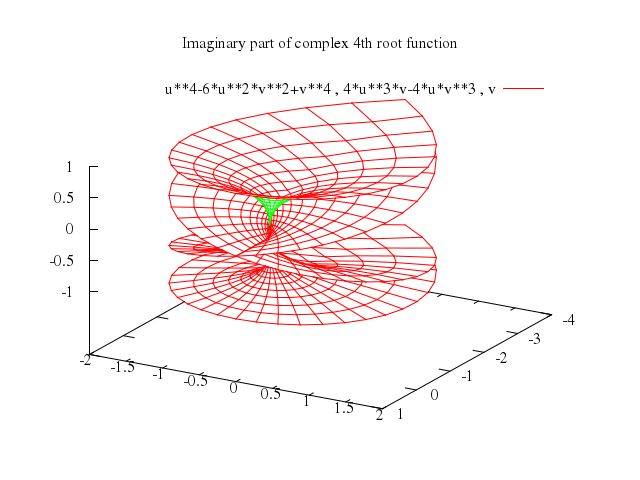
### 12
```ruby
# set view 60,300
# set title "Imaginary part of complex 4th root function (different view)"
# replot
Numo.gnuplot do
set view:[60,300]
set title:"Imaginary part of complex 4th root function (different view)"
replot
end
```
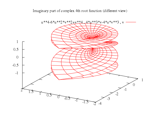
### 13
```ruby
# set isosamples 21
# set view 60,20
# set urange [-3:3]
# set vrange [-3:3]
# set title "Enneper's surface"
# splot u-u**3/3+u*v**2,v-v**3/3+v*u**2,u**2-v**2
Numo.gnuplot do
set isosamples:21
set view:[60,20]
set urange:-3..3
set vrange:-3..3
set title:"Enneper's surface"
splot "u-u**3/3+u*v**2",
"v-v**3/3+v*u**2",
"u**2-v**2"
end
```
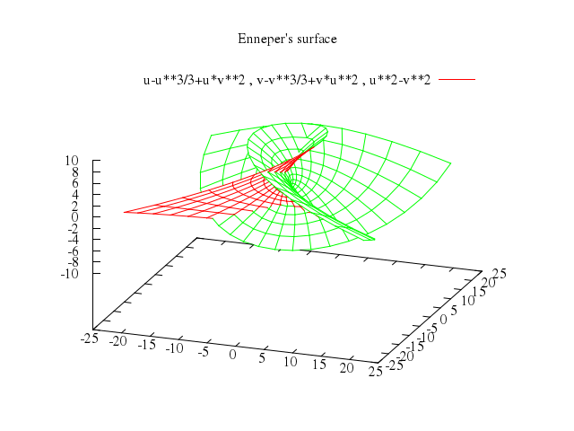
### 14
```ruby
# set view 60,110
# set title "Enneper's surface (different view)"
# replot
Numo.gnuplot do
set view:[60,110]
set title:"Enneper's surface (different view)"
replot
end
```
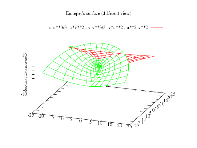
### 15
```ruby
# set isosamples 31,11
# set view 60,30
# set title "Moebius strip"
# set urange [0:2*pi]
# set vrange [-0.25:0.25]
# splot (2-v*sin(u/2))*sin(u),(2-v*sin(u/2))*cos(u),v*cos(u/2)
Numo.gnuplot do
set isosamples:[31,11]
set view:[60,30]
set title:"Moebius strip"
set urange:"[0:2*pi]"
set vrange:-0.25..0.25
splot "(2-v*sin(u/2))*sin(u)",
"(2-v*sin(u/2))*cos(u)",
"v*cos(u/2)"
end
```
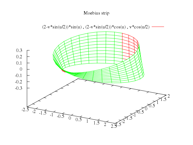
### 16
```ruby
# set view 60,210
# set title "Moebius strip (view from opposite side)"
# replot
Numo.gnuplot do
set view:[60,210]
set title:"Moebius strip (view from opposite side)"
replot
end
```
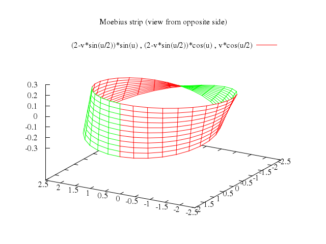
### 17
```ruby
# unset key
# set xrange [-10:10]
# set yrange [-10:10]
# set zrange [-3:3]
# set urange [0:2*pi]
# set vrange [0:2*pi]
# set isosamples 39,60
# set view 60,120
# set title "Klein bottle"
# splot (2*sin(u)*cos(v/2)-sin(2*u)*sin(v/2)+8)*cos(v), \
# (2*sin(u)*cos(v/2)-sin(2*u)*sin(v/2)+8)*sin(v), \
# 2*sin(u)*sin(v/2)+sin(2*u)*cos(v/2)
Numo.gnuplot do
unset :key
set xrange:-10..10
set yrange:-10..10
set zrange:-3..3
set urange:"[0:2*pi]"
set vrange:"[0:2*pi]"
set isosamples:[39,60]
set view:[60,120]
set title:"Klein bottle"
splot "(2*sin(u)*cos(v/2)-sin(2*u)*sin(v/2)+8)*cos(v)",
"(2*sin(u)*cos(v/2)-sin(2*u)*sin(v/2)+8)*sin(v)",
"2*sin(u)*sin(v/2)+sin(2*u)*cos(v/2)"
end
```
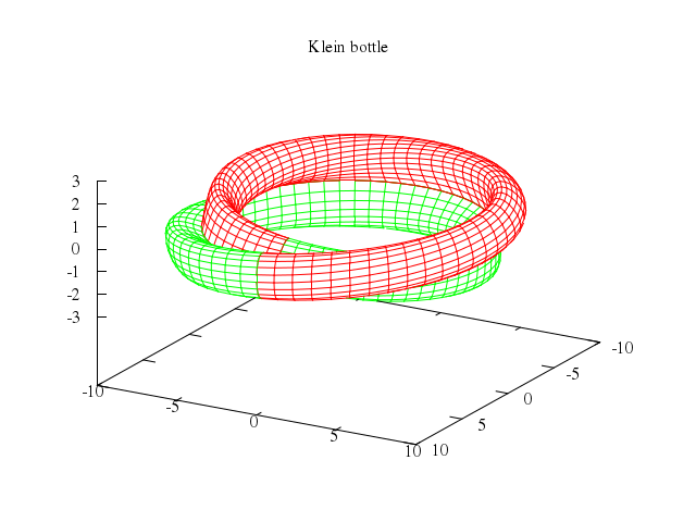
### 18
```ruby
# set urange [0:2*pi]
# set vrange [0:4*pi/3]
# set isosamples 39,40
# set view 60,20
# set title "Klein bottle with look at the 'inside'"
# replot
Numo.gnuplot do
set urange:"[0:2*pi]"
set vrange:"[0:4*pi/3]"
set isosamples:[39,40]
set view:[60,20]
set title:"Klein bottle with look at the 'inside'"
replot
end
```
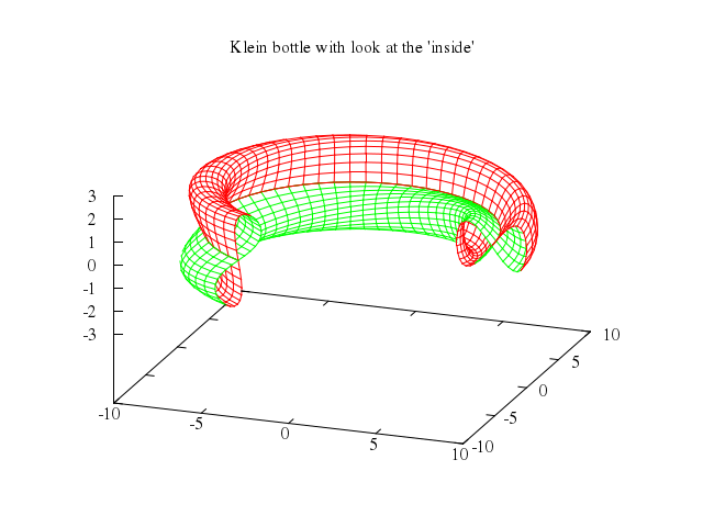
### 19
```ruby
# set style data lines
# set xrange [-12:12]
# set yrange [-12:12]
# set zrange [*:*]
# unset hidden3d
# set ticslevel 0.
# set view 50,15 #HBB: ,1,1.7
# set title "Klein bottle, glassblowers' version (look-through)"
# splot "klein.dat"
Numo.gnuplot do
set :style, :data, :lines
set xrange:-12..12
set yrange:-12..12
set zrange:"[*:*]"
unset :hidden3d
set ticslevel:0.0
set view:[50,15] #HBB: ,1,1.7
set title:"Klein bottle, glassblowers' version (look-through)"
splot "\"klein.dat\""
end
```
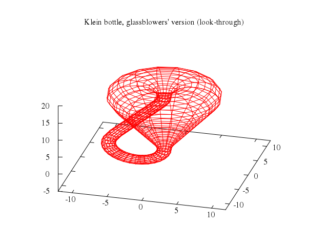
### 20
```ruby
# set hidden3d
# set view 70,305
# set title "Klein bottle, glassblowers' version (solid)"
# splot "klein.dat"
Numo.gnuplot do
set :hidden3d
set view:[70,305]
set title:"Klein bottle, glassblowers' version (solid)"
splot "\"klein.dat\""
end
```
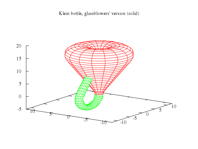
## hidden surfaces
[Original Demo](http://gnuplot.sourceforge.net/demo_4.6/hidden.html)
### 1
```ruby
# set samples 20
# set isosamples 20
# set hidden3d
# set title "Hidden line removal of explicit surfaces"
#
# set xrange [-3:3]
# set yrange [-2:2]
# splot 1 / (x*x + y*y + 1)
Numo.gnuplot do
set samples:20
set isosamples:20
set :hidden3d
set title:"Hidden line removal of explicit surfaces"
set xrange:-3..3
set yrange:-2..2
splot "1 / (x*x + y*y + 1)"
end
```
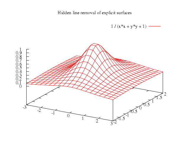
### 2
```ruby
# set xrange [-1:1]
# set yrange [-1:1]
# splot x*y / (x**2 + y**2 + 0.1)
Numo.gnuplot do
set xrange:-1..1
set yrange:-1..1
splot "x*y / (x**2 + y**2 + 0.1)"
end
```
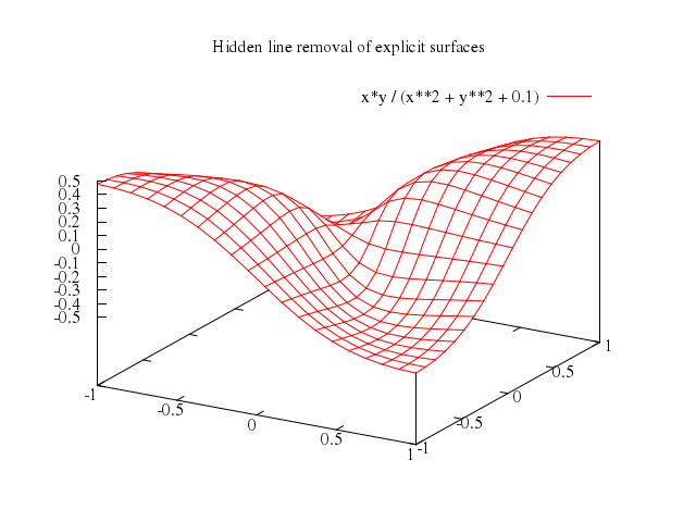
### 3
```ruby
# set view 70,45
# unset contour
# set xrange [-3:3]
# set yrange [-3:3]
# splot sin(x*x + y*y) / (x*x + y*y)
Numo.gnuplot do
set view:[70,45]
unset :contour
set xrange:-3..3
set yrange:-3..3
splot "sin(x*x + y*y) / (x*x + y*y)"
end
```
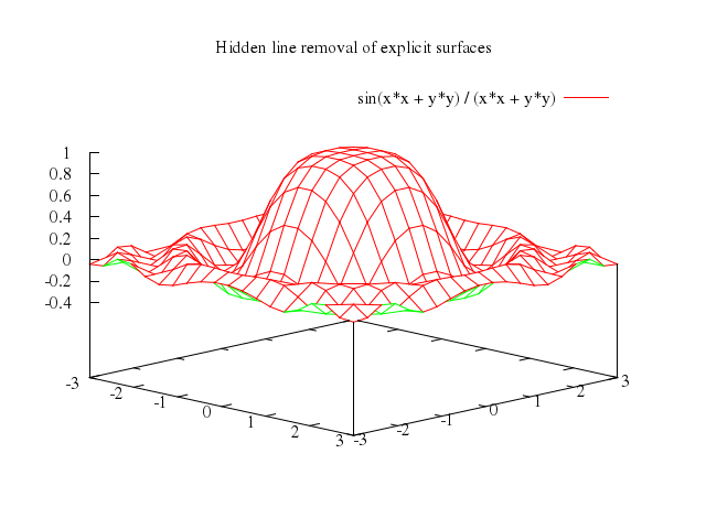
### 4
```ruby
# set view 60,30
# set xrange [-3:3]
# set yrange [-3:3]
# set zrange [-1:1]
# set ztics -1,0.5,1
# set grid z
# set border 4095
# splot sin(x) * cos(y)
Numo.gnuplot do
set view:[60,30]
set xrange:-3..3
set yrange:-3..3
set zrange:-1..1
set ztics:[-1,0.5,1]
set grid:"z"
set border:4095
splot "sin(x) * cos(y)"
end
```
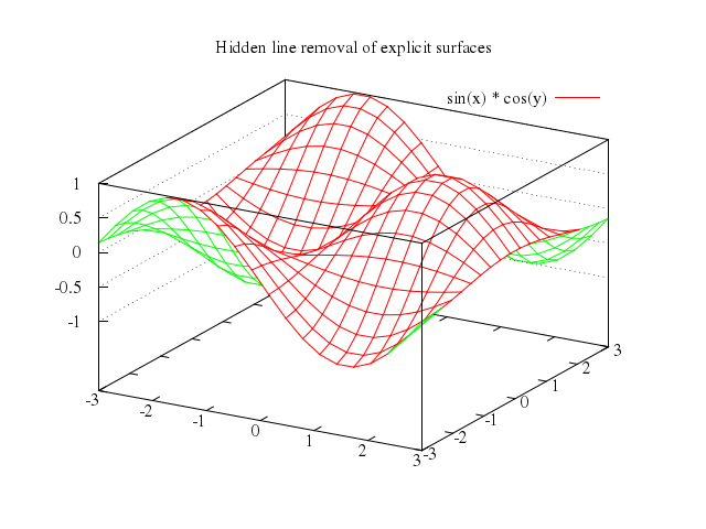
### 5
```ruby
# unset grid
# set ztics autofreq
# set border 31
# set view 75,230
# set contour
# replot
Numo.gnuplot do
unset :grid
set ztics:"autofreq"
set border:31
set view:[75,230]
set :contour
replot
end
```
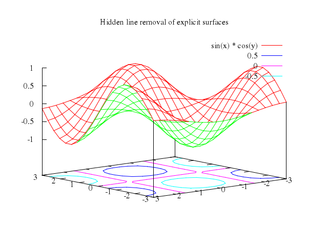
### 6
```ruby
# set view 80,30,1,1
# set style data lines
# # autoranging loses the verticals
# set xrange [0:15]
# set yrange [0:15]
# splot "glass.dat" using 1
Numo.gnuplot do
set view:[80,30,1,1]
set :style, :data, :lines
set xrange:0..15
set yrange:0..15
splot "\"glass.dat\"", using:1
end
```
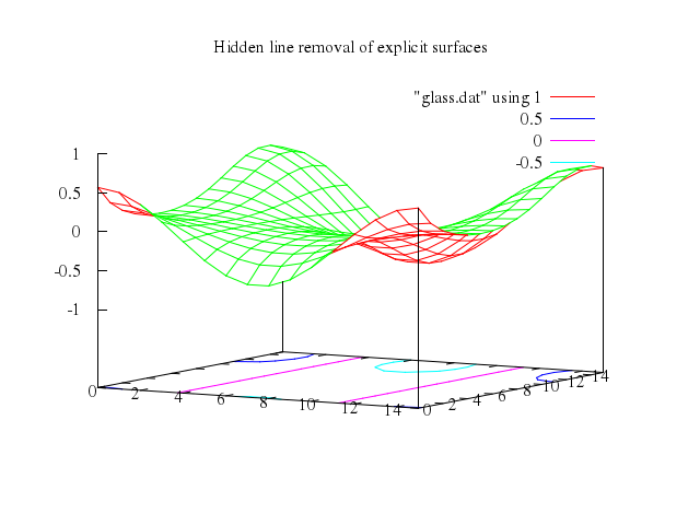
### 7
```ruby
# set view 50
# set grid
# replot
Numo.gnuplot do
set view:50
set :grid
replot
end
```
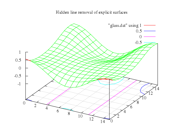
## pm3d coloring
[Original Demo](http://gnuplot.sourceforge.net/demo_4.6/pm3d.html)
### 1
```ruby
# # demo for pm3d splotting
# #
# # This demo can be directly used if your default terminal supports pm3d,
# # like OS/2 Presentation Manager, X11, Linux VGA, Windows.
# # Otherwise you can use the output to postscript, for example:
# # set term push; set term postscript color enhanced
# # set out 'pm3d_demo.ps'
# # load 'pm3d.dem'
# # set out; set term pop
#
# # Prepared by Petr Mikulik
# # History:
# # - 12. 3. 2003 pm: added demo for corners2color
# # - 9. 3. 2002 pm: added demo for ftriangles
# # - 31. 1. 2002 pm: removed pm3d/demo and stand-alone pm3d.dem in demo/
# # - 29. 1. 2002 joze: added demo for the 4th column
# # - 18. 3. 2001 pm: updated for cb-axis
# # - 18.11. 2000 pm: updated for 'set colorbox'
# # - 03. 3. 2000 joze: updated to show new pm3d features
# # - 15. 6. 1999 pm: update for `set pm3d`+`set palette`
# # - 29. 4. 1999 pm: the 1st version, directory pm3d/demo
#
# # print "WARNING: This demo works only on terminals supporting pm3d, i.e. on "
# # print "-------- OS/2 Presentation Manager, X11, Linux VGA, Windows. Please use"
# # print " output to a postscript file otherwise."
#
# set xlabel "x"
# set ylabel "y"
# set key top
# set border 4095
# set xrange [-15:15]
# set yrange [-15:15]
# set zrange [-0.25:1]
# set samples 25
# set isosamples 20
#
# set title "pm3d demo. Radial sinc function. Default options."
# set pm3d; set palette
# #show pm3d
# #show palette
# splot sin(sqrt(x**2+y**2))/sqrt(x**2+y**2)
Numo.gnuplot do
set xlabel:"x"
set ylabel:"y"
set :key, :top
set border:4095
set xrange:-15..15
set yrange:-15..15
set zrange:-0.25..1
set samples:25
set isosamples:20
set title:"pm3d demo. Radial sinc function. Default options."
set :pm3d; set :palette
splot "sin(sqrt(x**2+y**2))/sqrt(x**2+y**2)"
end
```
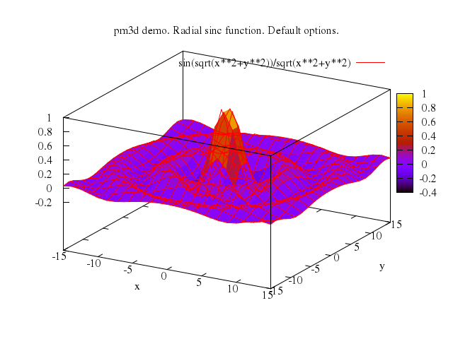
### 2
```ruby
# set title "pm3d at s (surface) / ticslevel 0"
# set ticslevel 0
# set pm3d at s
# set cblabel "colour gradient"
# replot
Numo.gnuplot do
set title:"pm3d at s (surface) / ticslevel 0"
set ticslevel:0
set :pm3d, :at, "s"
set cblabel:"colour gradient"
replot
end
```
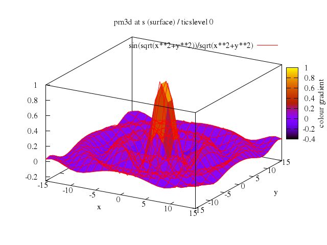
### 3
```ruby
# set title "pm3d at b (bottom)"
# set pm3d at b
# replot
Numo.gnuplot do
set title:"pm3d at b (bottom)"
set :pm3d, :at, "b"
replot
end
```
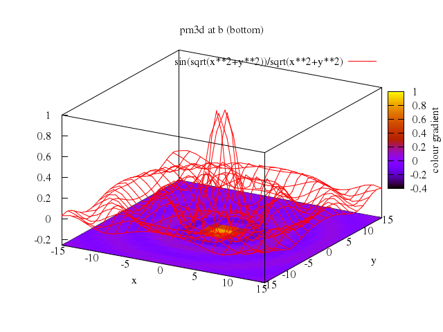
### 4
```ruby
# set title "unset surface; set pm3d at st (surface and top)"
# unset surface
# set pm3d at st
# replot
Numo.gnuplot do
set title:"unset surface; set pm3d at st (surface and top)"
unset :surface
set :pm3d, :at, "st"
replot
end
```
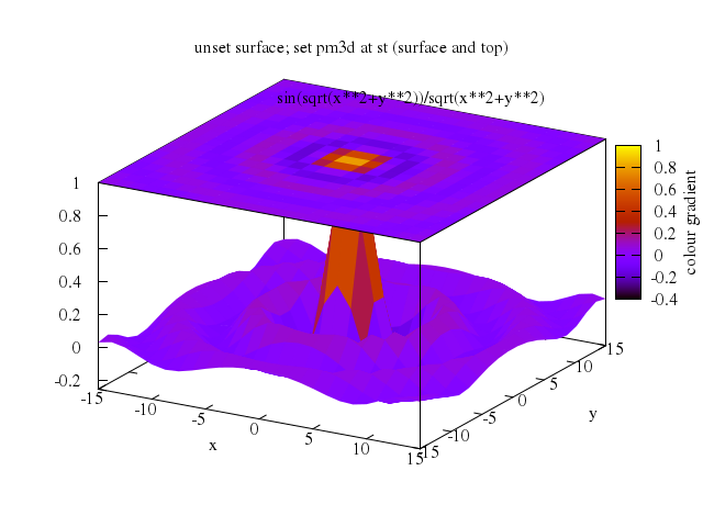
### 5
```ruby
# unset cblabel
#
# set title "set pm3d at bstbst (funny combination, only for screen or postscript)"
# set view 50,50
# set pm3d at bstbst
# replot
Numo.gnuplot do
unset :cblabel
set title:"set pm3d at bstbst (funny combination, only for screen or postscript)"
set view:[50,50]
set :pm3d, :at, "bstbst"
replot
end
```
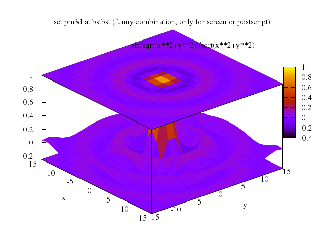
### 6
```ruby
# set title "gray map"
# set pm3d map
# set palette gray
# set samples 100; set isosamples 100
# replot
Numo.gnuplot do
set title:"gray map"
set :pm3d, :map
set :palette, "gray"
set samples:100; set isosamples:100
replot
end
```
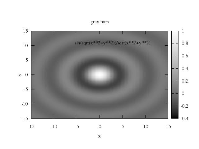
### 7
```ruby
# set title "gray map, negative"
# set pm3d map
# set palette gray negative
# replot
Numo.gnuplot do
set title:"gray map, negative"
set :pm3d, :map
set :palette, "gray negative"
replot
end
```
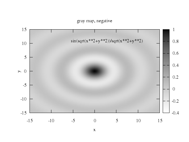
### 8
```ruby
# set title "colour map, using default rgbformulae 7,5,15 ... traditional pm3d (black-blue-red-yellow)"
# set palette color positive
# set pm3d map
# set samples 50; set isosamples 50
# replot
Numo.gnuplot do
set title:"colour map, using default rgbformulae 7,5,15 ... traditional pm3d (black-blue-red-yellow)"
set :palette, color:"positive"
set :pm3d, :map
set samples:50; set isosamples:50
replot
end
```
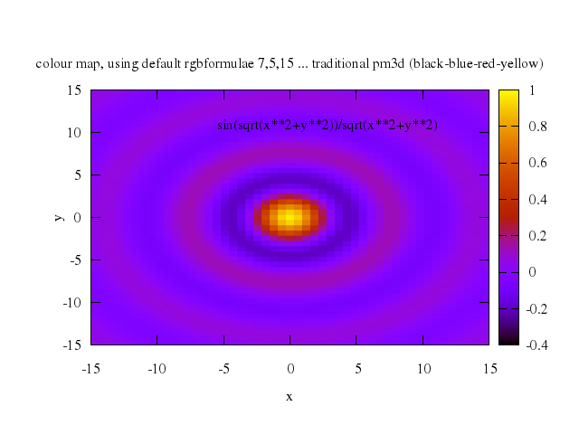
### 9
```ruby
# set title "colour, rgbformulae 3,11,6 ... green-red-violet"
# set palette rgbformulae 3,11,6
# replot
Numo.gnuplot do
set title:"colour, rgbformulae 3,11,6 ... green-red-violet"
set :palette, rgbformulae:[3,11,6]
replot
end
```
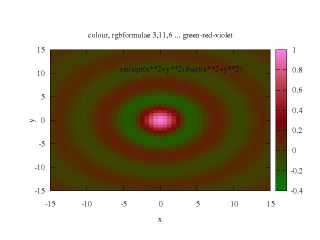
### 10
```ruby
# set title "colour, rgbformulae 23,28,3 ... ocean (green-blue-white); OK are also all other permutations"
# set palette rgbformulae 23,28,3
# replot
Numo.gnuplot do
set title:"colour, rgbformulae 23,28,3 ... ocean (green-blue-white); OK are also all other permutations"
set :palette, rgbformulae:[23,28,3]
replot
end
```
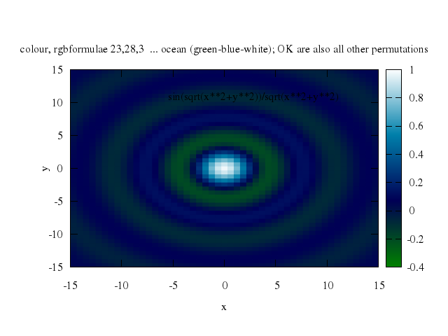
### 11
```ruby
# set title "colour, rgbformulae 30,31,32 ... color printable on gray (black-blue-violet-yellow-white)"
# set palette rgbformulae 30,31,32
# replot
Numo.gnuplot do
set title:"colour, rgbformulae 30,31,32 ... color printable on gray (black-blue-violet-yellow-white)"
set :palette, rgbformulae:[30,31,32]
replot
end
```
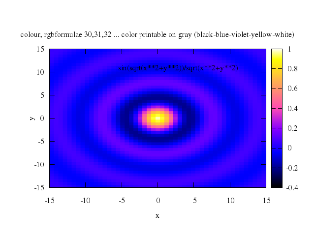
### 12
```ruby
# set title "cubehelix color scheme with monotonic intensity\nD A Green (2011) http://arxiv.org/abs/1108.5083" offset 0,1
# set palette cubehelix
# replot
Numo.gnuplot do
set title:"cubehelix color scheme with monotonic intensity\nD A Green (2011) http://arxiv.org/abs/1108.5083", offset:[0,1]
set :palette, :cubehelix
replot
end
```
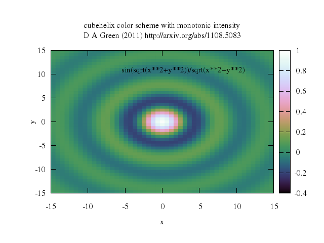
### 13
```ruby
# #test palette
# #pause -1 "Hit return to continue"
#
# set title "rgbformulae 31,-11,32: negative formula number=inverted color"
# set palette rgbformulae 31,-11,32
# replot
Numo.gnuplot do
set title:"rgbformulae 31,-11,32: negative formula number=inverted color"
set :palette, rgbformulae:[31,-11,32]
replot
end
```
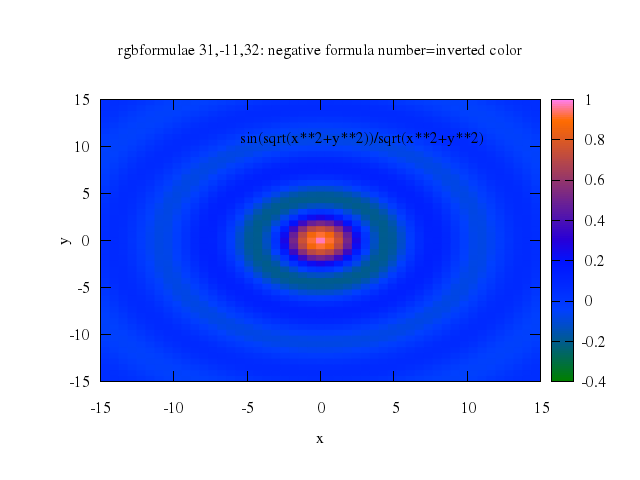
### 14
```ruby
# set yrange [*:*] noreverse
#
# reset
#
# set title "set pm3d scansforward: wrong, because back overwrites front"
# set pm3d
# set palette
# set view 130,10
# set samples 50; set isosamples 50
# set border 4095
# unset surface
# set pm3d at s scansforward
# splot sin(sqrt(x**2+y**2))/sqrt(x**2+y**2)
Numo.gnuplot do
set yrange:"[*:*]", noreverse:true
reset
set title:"set pm3d scansforward: wrong, because back overwrites front"
set :pm3d
set :palette
set view:[130,10]
set samples:50; set isosamples:50
set border:4095
unset :surface
set :pm3d, :at, "s", "scansforward"
splot "sin(sqrt(x**2+y**2))/sqrt(x**2+y**2)"
end
```
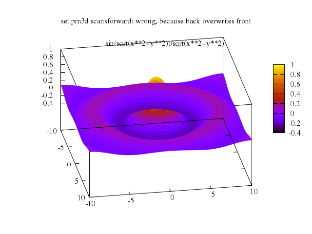
### 15
```ruby
# set title "set pm3d scansbackward: correctly looking surface"
# set xlabel
# set border 4095
# set pm3d scansbackward
# replot
Numo.gnuplot do
set title:"set pm3d scansbackward: correctly looking surface"
set :xlabel
set border:4095
set pm3d:"scansbackward"
replot
end
```
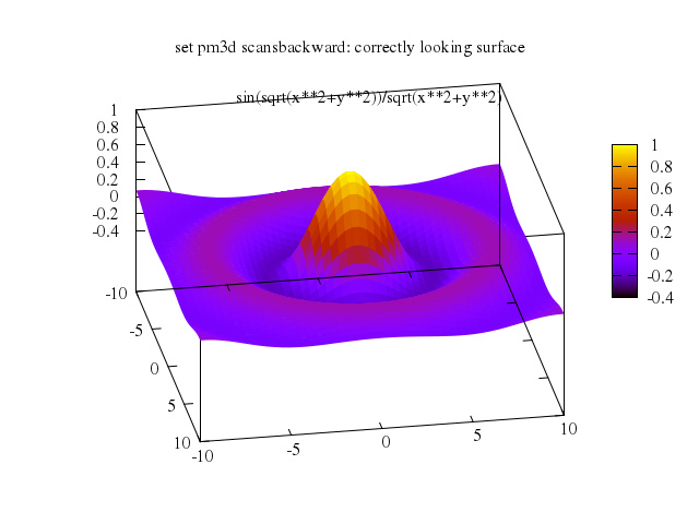
### 16
```ruby
# set title "set hidden3d"
# set samples 30; set isosamples 30
# set hidden3d
# set pm3d
# set surface
# set view 50,220
# set xrange [-2:2]
# set yrange [-2:2]
# splot log(x*x*y*y)
Numo.gnuplot do
set title:"set hidden3d"
set samples:30; set isosamples:30
set :hidden3d
set :pm3d
set :surface
set view:[50,220]
set xrange:-2..2
set yrange:-2..2
splot "log(x*x*y*y)"
end
```
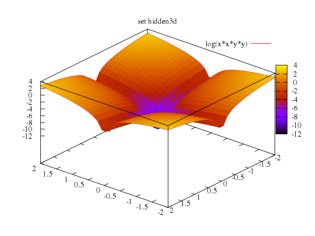
### 17
```ruby
# unset hidden3d
#
# # draw the surface using pm3d's hidden3d with line type 100
# unset hidden
# unset surface
#
# set title "set pm3d hidden3d : pm3d's much faster hidden3d variant"
# set samples 30; set isosamples 30
# set pm3d
# set style line 100 lt 5 lw 0.5
# set pm3d hidden3d 100
# set view 50,220
# set xrange [-2:2]
# set yrange [-2:2]
# splot log(x*x*y*y)
Numo.gnuplot do
unset :hidden3d
unset :hidden
unset :surface
set title:"set pm3d hidden3d : pm3d's much faster hidden3d variant"
set samples:30; set isosamples:30
set :pm3d
set :style, :line, 100, lt:5, lw:0.5
set :pm3d, :hidden3d, 100
set view:[50,220]
set xrange:-2..2
set yrange:-2..2
splot "log(x*x*y*y)"
end
```
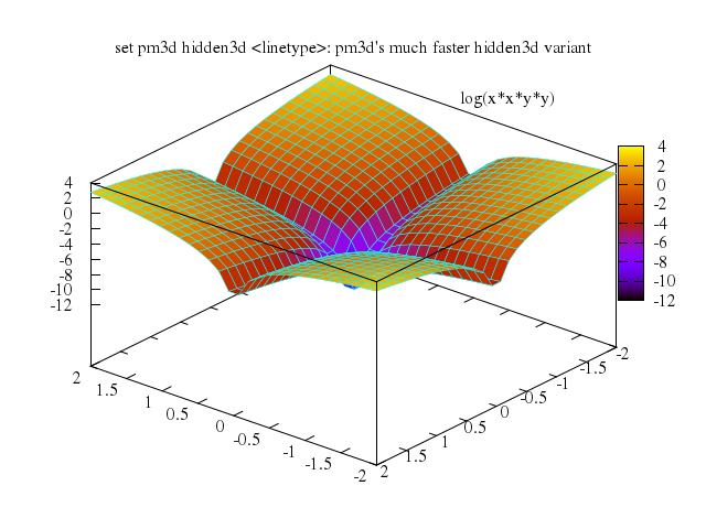
### 18
```ruby
# set pm3d nohidden3d
#
# set title "bad: surface and top are too close together"
# set xrange [-1:1]
# set yrange [-1:1]
# unset hidd
# set zrange [-15:4]
# set ticslevel 0
# set pm3d at st
# splot log(x*x*y*y)
Numo.gnuplot do
set :pm3d, :nohidden3d
set title:"bad: surface and top are too close together"
set xrange:-1..1
set yrange:-1..1
unset :hidd
set zrange:-15..4
set ticslevel:0
set :pm3d, :at, "st"
splot "log(x*x*y*y)"
end
```
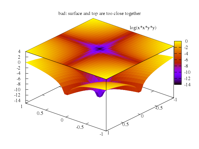
### 19
```ruby
# set title "solution: use independent 'set zrange' and 'set cbrange'"
# unset surf
# set cbrange [-15:4]
# set zrange [-15:60]
# splot log(x*x*y*y)
Numo.gnuplot do
set title:"solution: use independent 'set zrange' and 'set cbrange'"
unset :surf
set cbrange:-15..4
set zrange:-15..60
splot "log(x*x*y*y)"
end
```
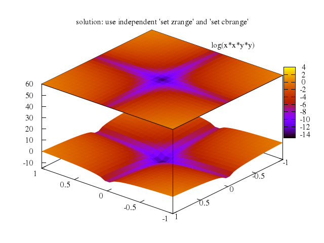
### 20
```ruby
# set autoscale cb
#
# set title "color box is on by default at a certain position"
# set samples 20; set isosamples 20
# set autoscale
# set key on
# set pm3d
# set pm3d at s
# set view 60,30
# splot y
Numo.gnuplot do
set :autoscale, :cb
set title:"color box is on by default at a certain position"
set samples:20; set isosamples:20
set :autoscale
set :key, :on
set :pm3d
set :pm3d, :at, "s"
set view:[60,30]
splot "y"
end
```
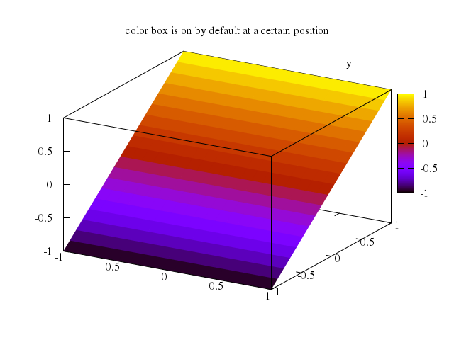
### 21
```ruby
# set title "color box is on again, now with horizontal gradient"
# set size 0.6,0.6; set origin 0.2,0.25
# set colorbox horizontal
# set colorbox user origin 0.1,0.15 size 0.8,0.1
# set mcbtics 2
# set grid cb
# set cblabel "see cblabel, grid cb, mcbtics, ..."
# replot
Numo.gnuplot do
set title:"color box is on again, now with horizontal gradient"
set size:[0.6,0.6]; set origin:[0.2,0.25]
set :colorbox, :horizontal
set :colorbox, "user", origin:[0.1,0.15], size:[0.8,0.1]
set "mcbtics", 2
set :grid, :cb
set cblabel:"see cblabel, grid cb, mcbtics, ..."
replot
end
```
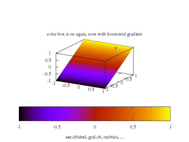
### 22
```ruby
# unset cblabel; unset mcbtics; set grid nocb; set colorbox default
#
# set title "color box is switched off"
# unset colorbox
# replot
Numo.gnuplot do
unset :cblabel; unset :mcbtics; set :grid, :nocb; set :colorbox, :default
set title:"color box is switched off"
unset :colorbox
replot
end
```
### 23
```ruby
# set title 'using now "set grid back; unset colorbox"'
# unset colorbox
# set pm3d
# set border 895
# set grid back
# replot
Numo.gnuplot do
set title:'using now "set grid back; unset colorbox"'
unset :colorbox
set :pm3d
set border:895
set :grid, :back
replot
end
```

### 24
```ruby
# set size 1,1; set origin 0,0
# set grid layerdefault
# set xlabel "X LABEL"
# set ylabel "Y LABEL"
#
# set sample 11; set isosamples 11
# set pm3d map
# set palette
# set colorbox
# set lmargin 0
#
# set pm3d flush begin
# set title "Datafile with different nb of points in scans; pm3d flush begin"
# set pm3d flush begin noftriangles scansforward
# splot 'triangle.dat'
Numo.gnuplot do
set size:[1,1]; set origin:[0,0]
set grid:"layerdefault"
set xlabel:"X LABEL"
set ylabel:"Y LABEL"
set sample:11; set isosamples:11
set :pm3d, :map
set :palette
set :colorbox
set lmargin:0
set :pm3d, "flush begin"
set title:"Datafile with different nb of points in scans; pm3d flush begin"
set :pm3d, "flush begin noftriangles scansforward"
splot "'triangle.dat'"
end
```
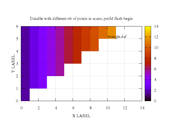
### 25
```ruby
# #show pm3d
#
# set title "Datafile with different nb of points in scans; pm3d flush center"
# set pm3d flush center scansforward
# replot
Numo.gnuplot do
set title:"Datafile with different nb of points in scans; pm3d flush center"
set :pm3d, "flush", center:"scansforward"
replot
end
```

### 26
```ruby
# set title "Datafile with different nb of points in scans; pm3d flush end"
# set pm3d flush end scansforward
# replot
Numo.gnuplot do
set title:"Datafile with different nb of points in scans; pm3d flush end"
set :pm3d, "flush end scansforward"
replot
end
```
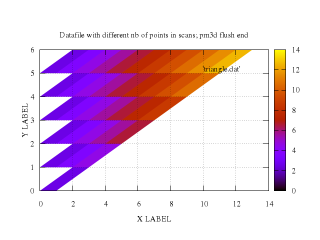
### 27
```ruby
# set grid front
#
# set pm3d flush begin
# set title "Data with different nb of points in scans; pm3d ftriangles flush begin"
# set pm3d flush begin ftriangles scansforward
# splot 'triangle.dat'
Numo.gnuplot do
set :grid, :front
set :pm3d, "flush begin"
set title:"Data with different nb of points in scans; pm3d ftriangles flush begin"
set :pm3d, "flush begin ftriangles scansforward"
splot "'triangle.dat'"
end
```

### 28
```ruby
# #show pm3d
#
# set title "Data with different nb of points in scans; pm3d ftriangles flush center"
# set pm3d flush center ftriangles scansforward
# replot
Numo.gnuplot do
set title:"Data with different nb of points in scans; pm3d ftriangles flush center"
set :pm3d, "flush", center:"ftriangles scansforward"
replot
end
```
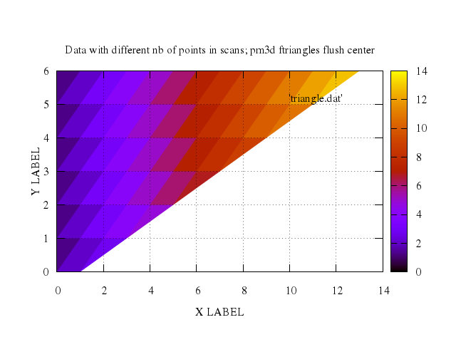
### 29
```ruby
# set title "Data with different nb of points in scans; pm3d ftriangles flush end"
# set pm3d flush end ftriangles scansforward
# replot
Numo.gnuplot do
set title:"Data with different nb of points in scans; pm3d ftriangles flush end"
set :pm3d, "flush end ftriangles scansforward"
replot
end
```

### 30
```ruby
# set title "Using interpolation with datafile; pm3d map interpolate 2,1"
# set pm3d flush begin noftriangles scansforward interpolate 2,1
# replot
Numo.gnuplot do
set title:"Using interpolation with datafile; pm3d map interpolate 2,1"
set :pm3d, "flush begin noftriangles scansforward", interpolate:[2,1]
replot
end
```

### 31
```ruby
# set title "Using interpolation with datafile; pm3d map ftriangles interpolate 10,1"
# set pm3d flush begin ftriangles scansforward interpolate 10,1
# replot
Numo.gnuplot do
set title:"Using interpolation with datafile; pm3d map ftriangles interpolate 10,1"
set :pm3d, "flush begin ftriangles scansforward", interpolate:[10,1]
replot
end
```

### 32
```ruby
# set title "Using interpolation with datafile; pm3d at s ftriangles interpolate 10,1"
# set pm3d flush begin ftriangles scansforward at s interpolate 10,1
# set view 20,20
# replot
Numo.gnuplot do
set title:"Using interpolation with datafile; pm3d at s ftriangles interpolate 10,1"
set :pm3d, "flush begin ftriangles scansforward", at:"s", interpolate:[10,1]
set view:[20,20]
replot
end
```
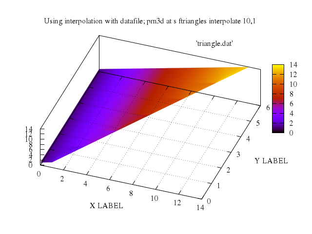
### 33
```ruby
# reset
#
# set title "only for enhanced terminals: 'set format cb ...'"
# set xlabel "X"
# set ylabel "Y"
# set sample 31; set isosamples 31
# set xrange [-185:185]
# set yrange [-185:185]
# set format cb "%.01t*10^{%T}"
# unset surface
# set border 4095
# set ticslevel 0
# set pm3d at s; set palette gray
# set cblabel "the colour gradient"
# splot abs(x)**3+abs(y)**3
Numo.gnuplot do
reset
set title:"only for enhanced terminals: 'set format cb ...'"
set xlabel:"X"
set ylabel:"Y"
set sample:31; set isosamples:31
set xrange:-185..185
set yrange:-185..185
set format_cb:"%.01t*10^{%T}"
unset :surface
set border:4095
set ticslevel:0
set :pm3d, :at, "s"; set :palette, "gray"
set cblabel:"the colour gradient"
splot "abs(x)**3+abs(y)**3"
end
```
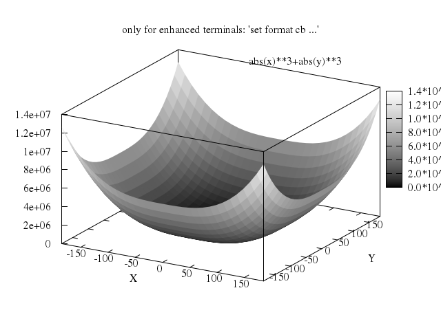
### 34
```ruby
# unset cblabel
#
# set pal color
# set xrange [*:*]; set yrange [*:*]
# set title "function 'x+y' using all colors available, 'set pal maxcolors 0'"
# set pal maxcolors 0
# splot x+y
Numo.gnuplot do
unset :cblabel
set :pal, :color
set xrange:"[*:*]"; set yrange:"[*:*]"
set title:"function 'x+y' using all colors available, 'set pal maxcolors 0'"
set :pal, maxcolors:0
splot "x+y"
end
```
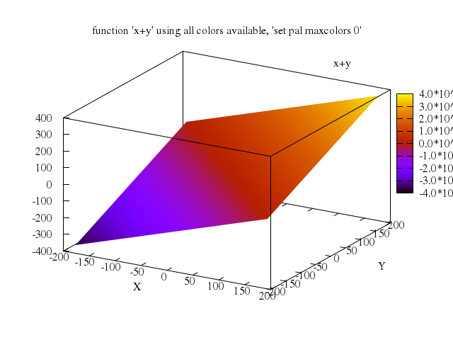
### 35
```ruby
# set xrange [*:*]; set yrange [*:*]
# set title "function 'x+y' using only 5 colors, 'set pal maxcolors 5'"
# set pal maxcolors 5
# splot x+y
Numo.gnuplot do
set xrange:"[*:*]"; set yrange:"[*:*]"
set title:"function 'x+y' using only 5 colors, 'set pal maxcolors 5'"
set :pal, maxcolors:5
splot "x+y"
end
```
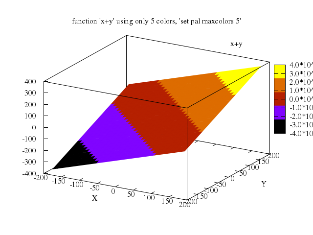
### 36
```ruby
# set pal maxcolors 0
# unset pm3d
# set surface
# set format z
# set palette
# set title "color lines: 'splot sin(y)/(y) with lines palette'"
# set ticslevel 0
# set border 4095
# set xrange [-10:10]; set yrange [-10:10]
# set hidden3d
# set isosamples 40,40; set samples 40,40
# splot sin(y)/(y) w lines palette
Numo.gnuplot do
set :pal, maxcolors:0
unset :pm3d
set :surface
set format:"z"
set :palette
set title:"color lines: 'splot sin(y)/(y) with lines palette'"
set ticslevel:0
set border:4095
set xrange:-10..10; set yrange:-10..10
set :hidden3d
set isosamples:[40,40]; set samples:[40,40]
splot "sin(y)/(y)", w:"lines", palette:true
end
```
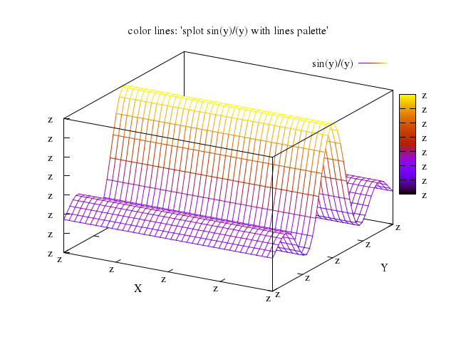
### 37
```ruby
# reset
#
# set title "Demo for clipping of 2 rectangles comes now. The xrange is [0:2]..."
# set pm3d; set palette
# set pm3d map
#
# set xrange [0:2]
# splot 'clip14in.dat'
Numo.gnuplot do
reset
set title:"Demo for clipping of 2 rectangles comes now. The xrange is [0:2]..."
set :pm3d; set :palette
set :pm3d, :map
set xrange:0..2
splot "'clip14in.dat'"
end
```
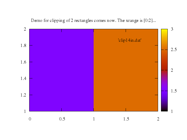
### 38
```ruby
# set xrange [0:1.5]
# set yrange [*:*]
# set title "...and now xrange is [0:1.5] and 'set pm3d clip1in'"
# set pm3d clip1in
# replot
Numo.gnuplot do
set xrange:0..1.5
set yrange:"[*:*]"
set title:"...and now xrange is [0:1.5] and 'set pm3d clip1in'"
set pm3d:"clip1in"
replot
end
```
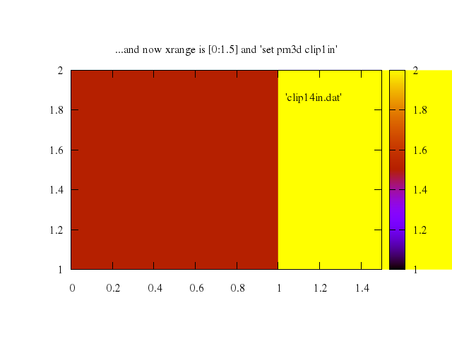
### 39
```ruby
# set title "...now xrange is [0:1.5] and 'set pm3d clip4in'"
# set pm3d clip4in
# replot
Numo.gnuplot do
set title:"...now xrange is [0:1.5] and 'set pm3d clip4in'"
set pm3d:"clip4in"
replot
end
```
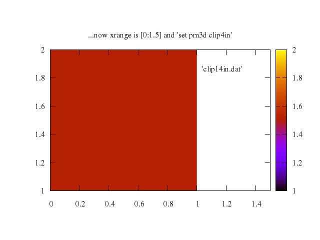
### 40
```ruby
# reset
#
# sinc(u,v) = sin(sqrt(u**2+v**2)) /sqrt(u**2+v**2)
#
# set sam 40
# set iso 40
#
# set title "pm3d explicit mode --- coloring according to the 4th parameter of 'using'"
# set ticslevel 0
#
# set pm3d at s explicit
#
# # 'binary2' binary u 1:2:(column(3)+column(-1)/20.0):3 w pm3d,
#
# splot \
# 'binary2' binary u 1:2:3:($2+($1+$2)/10) w pm3d, \
# 1+sinc(x*4, y*4) w l
Numo.gnuplot do
reset
run "sinc(u,v) = sin(sqrt(u**2+v**2)) /sqrt(u**2+v**2)"
set sam:40
set iso:40
set title:"pm3d explicit mode --- coloring according to the 4th parameter of 'using'"
set ticslevel:0
set :pm3d, :at, "s", "explicit"
splot ["'binary2'", :binary, u:'1:2:3:($2+($1+$2)/10)', w:"pm3d"],
["1+sinc(x*4, y*4)", w:"l"]
end
```
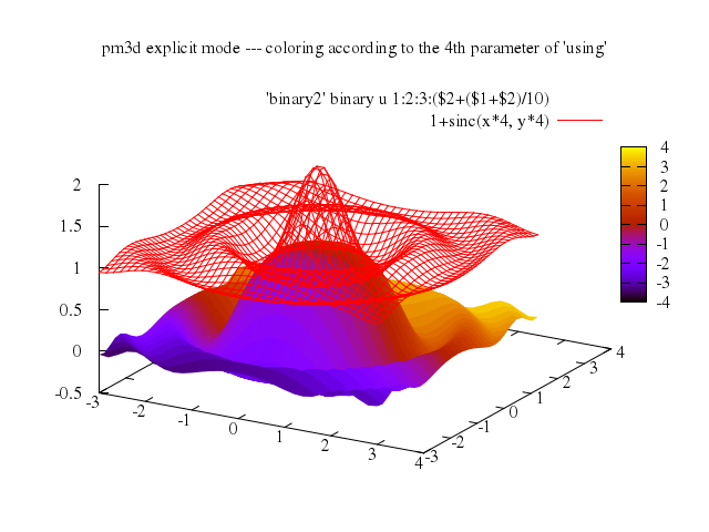
### 41
```ruby
# set title "coloring according to the 3rd 'using' parameter (left) and to the z-value (bottom)"
# set border 895
# splot \
# 'binary2' binary u 2:(12 - column(3) * 10):1 notitle w lines, \
# 'binary2' binary u (-12 + column(3) * 10):2:1:(-12 + column(3) * 10) notitle w pm3d, \
# 'binary2' binary u 1:2:(column(3) * 10 - 12) notitle w pm3d
Numo.gnuplot do
set title:"coloring according to the 3rd 'using' parameter (left) and to the z-value (bottom)"
set border:895
splot ["'binary2'", :binary, u:'2:(12 - column(3) * 10):1', notitle:true, w:"lines"],
["'binary2'", :binary, u:'(-12 + column(3) * 10):2:1:(-12 + column(3) * 10)', notitle:true, w:"pm3d"],
["'binary2'", :binary, u:'1:2:(column(3) * 10 - 12)', notitle:true, w:"pm3d"]
end
```
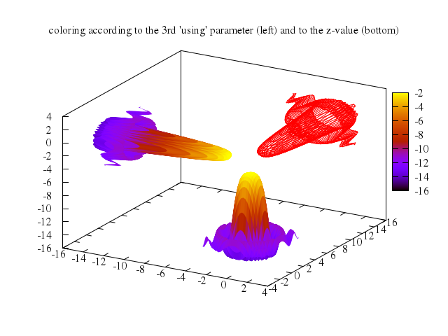
### 42
```ruby
# reset
#
# print "Plot by pm3d algorithm draws quadrangles filled with color calculated from"
# print "the z- or color-value of the surrounding 4 corners. The following demo shows"
# print "different color spots for a plot with very small number of quadrangles (here"
# print "rectangular pixels). Note that the default option is 'mean'."
#
# set pm3d map
# set iso 4
# set samples 4
# set xrange [0:3]
# set yrange [0:3]
# set cbrange [0:9]
# f(x,y)=2*x+y
# set key off
# unset xtics
# unset ytics
# set tics scale 2
# set colorbox horizontal user origin 0.1,0.025 size .8,0.02
#
# # Needed by terminals limited on colors:
# #set palette maxcolors 26
#
# # Note: no more space in the following multiplot to show demo for
# #set pm3d corners2color median
# #set pm3d corners2color geomean
#
# set multiplot
# # Let us do multiplot grid 3x3:
# dx = 1.0/3; dy = 1.0/3;
# set size dx,dy
#
# set origin 0*dx,0*dy
# set title "set pm3d corners2color c1"
# set pm3d corners2color c1
# splot f(x,y)
#
# set origin 2*dx,0*dy
# set title "set pm3d corners2color c2"
# set pm3d corners2color c2
# replot
#
# set origin 0*dx,2*dy
# set title "set pm3d corners2color c3"
# set pm3d corners2color c3
# replot
#
# set origin 2*dx,2*dy
# set title "set pm3d corners2color c4"
# set pm3d corners2color c4
# replot
#
# set origin 0*dx,1*dy
# set title "set pm3d corners2color mean"
# set pm3d corners2color mean
# replot
#
# set origin 2*dx,1*dy
# set title "set pm3d corners2color geomean"
# set pm3d corners2color geomean
# replot
#
# set origin 1*dx,0*dy
# set title "set pm3d corners2color median"
# set pm3d corners2color median
# replot
#
# set origin 1*dx,1*dy
# set title "Original grid points"
# unset pm3d
# set border 0
# unset xtics
# unset ytics
# unset colorbox
# #splot x*2+y with points ps 3 pt 5 palette
# splot f(x,y) with linesp ps 3 pt 5 palette
#
# unset multiplot
Numo.gnuplot do
reset
set :pm3d, :map
set iso:4
set samples:4
set xrange:0..3
set yrange:0..3
set cbrange:0..9
run "f(x,y)=2*x+y"
set :key, :off
unset :xtics
unset :ytics
set :tics, :scale, 2
set :colorbox, :horizontal, "user", origin:[0.1,0.025], size:[0.8,0.02]
set :multiplot
run "dx = 1.0/3; dy = 1.0/3;"
set size:"dx,dy"
set origin:'0*dx,0*dy'
set title:"set pm3d corners2color c1"
set :pm3d, "corners2color c1"
splot "f(x,y)"
set origin:'2*dx,0*dy'
set title:"set pm3d corners2color c2"
set :pm3d, "corners2color c2"
replot
set origin:'0*dx,2*dy'
set title:"set pm3d corners2color c3"
set :pm3d, "corners2color c3"
replot
set origin:'2*dx,2*dy'
set title:"set pm3d corners2color c4"
set :pm3d, "corners2color c4"
replot
set origin:'0*dx,1*dy'
set title:"set pm3d corners2color mean"
set :pm3d, "corners2color mean"
replot
set origin:'2*dx,1*dy'
set title:"set pm3d corners2color geomean"
set :pm3d, "corners2color geomean"
replot
set origin:'1*dx,0*dy'
set title:"set pm3d corners2color median"
set :pm3d, "corners2color median"
replot
set origin:'1*dx,1*dy'
set title:"Original grid points"
unset :pm3d
set border:0
unset :xtics
unset :ytics
unset :colorbox
splot "f(x,y)", with:"linesp", ps:3, pt:5, palette:true
unset :multiplot
end
```
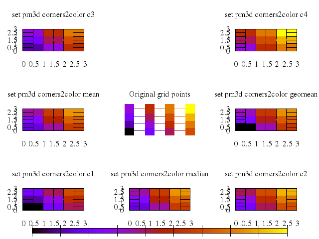
## pm3d hidden surfaces
[Original Demo](http://gnuplot.sourceforge.net/demo_4.6/hidden2.html)
### 1
```ruby
# # PM3D surfaces are not fully included in the calculation of hidden line removal.
# # Older versions of gnuplot allowed you to approximate the correct occlusion
# # by drawing the surface twice, once "with pm3d" to produce the surface you
# # want to show, and once "with lines lt -2" to include the same surface in
# # hidden3d calculations but drawn with invisible lines.
# # Current gnuplot does the approximation for you so the extra copy of the
# # surface is no longer necessary.
# #
# set isosamples 25,25
# set xyplane at 0
# unset key
#
# set palette rgbformulae 31,-11,32
# set style fill solid 0.5
# set cbrange [-1:1]
#
# set title "Mixing pm3d surfaces with hidden-line plots"
#
# f(x,y) = sin(-sqrt((x+5)**2+(y-7)**2)*0.5)
#
# set hidden3d front
# splot f(x,y) with pm3d, x*x-y*y with lines lc rgb "black"
Numo.gnuplot do
set isosamples:[25,25]
set :xyplane, at:0
unset :key
set :palette, rgbformulae:[31,-11,32]
set :style, fill_solid:0.5
set cbrange:-1..1
set title:"Mixing pm3d surfaces with hidden-line plots"
run "f(x,y) = sin(-sqrt((x+5)**2+(y-7)**2)*0.5)"
set :hidden3d, :front
splot ["f(x,y)", with:"pm3d"],
["x*x-y*y", with:"lines", lc_rgb:"black"]
end
```
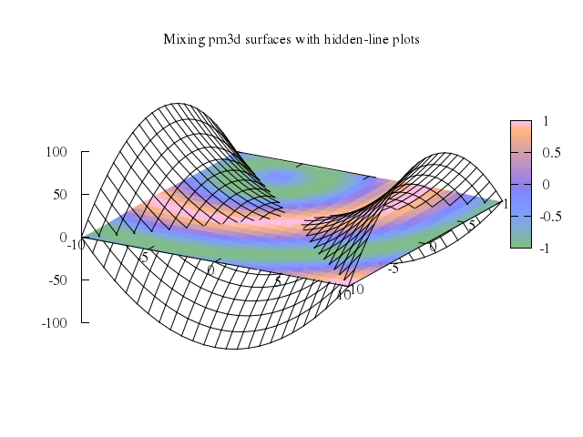
### 2
```ruby
# reset
#
# #
# # Another example of pm3d hidden surface removal,
# # this time using pm3d depth-ordering
# #
# set multiplot title "Interlocking Tori"
# set title "PM3D surface\nno depth sorting"
#
# set parametric
# set urange [-pi:pi]
# set vrange [-pi:pi]
# set isosamples 50,20
#
# set origin -0.02,0.0
# set size 0.55, 0.9
#
# unset key
# unset xtics
# unset ytics
# unset ztics
# set border 0
# set view 60, 30, 1.5, 0.9
# unset colorbox
#
# set pm3d scansbackward
# splot cos(u)+.5*cos(u)*cos(v),sin(u)+.5*sin(u)*cos(v),.5*sin(v) with pm3d, \
# 1+cos(u)+.5*cos(u)*cos(v),.5*sin(v),sin(u)+.5*sin(u)*cos(v) with pm3d
#
# set title "PM3D surface\ndepth sorting"
#
# set origin 0.40,0.0
# set size 0.55, 0.9
# set colorbox vertical user origin 0.9, 0.15 size 0.02, 0.50
# set format cb "%.1f"
#
# set pm3d depthorder
# splot cos(u)+.5*cos(u)*cos(v),sin(u)+.5*sin(u)*cos(v),.5*sin(v) with pm3d, \
# 1+cos(u)+.5*cos(u)*cos(v),.5*sin(v),sin(u)+.5*sin(u)*cos(v) with pm3d
#
# unset multiplot
Numo.gnuplot do
reset
set :multiplot, title:"Interlocking Tori"
set title:"PM3D surface\nno depth sorting"
set :parametric
set urange:"[-pi:pi]"
set vrange:"[-pi:pi]"
set isosamples:[50,20]
set origin:[-0.02,0.0]
set size:[0.55,0.9]
unset :key
unset :xtics
unset :ytics
unset :ztics
set border:0
set view:[60,30,1.5,0.9]
unset :colorbox
set pm3d:"scansbackward"
splot "cos(u)+.5*cos(u)*cos(v)",
"sin(u)+.5*sin(u)*cos(v)",
[".5*sin(v)", with:"pm3d"],
"1+cos(u)+.5*cos(u)*cos(v)",
".5*sin(v)",
["sin(u)+.5*sin(u)*cos(v)", with:"pm3d"]
set title:"PM3D surface\ndepth sorting"
set origin:[0.40,0.0]
set size:[0.55,0.9]
set :colorbox, :vertical, "user", origin:[0.9,0.15], size:[0.02,0.50]
set format_cb:"%.1f"
set pm3d:"depthorder"
splot "cos(u)+.5*cos(u)*cos(v)",
"sin(u)+.5*sin(u)*cos(v)",
[".5*sin(v)", with:"pm3d"],
"1+cos(u)+.5*cos(u)*cos(v)",
".5*sin(v)",
["sin(u)+.5*sin(u)*cos(v)", with:"pm3d"]
unset :multiplot
end
```
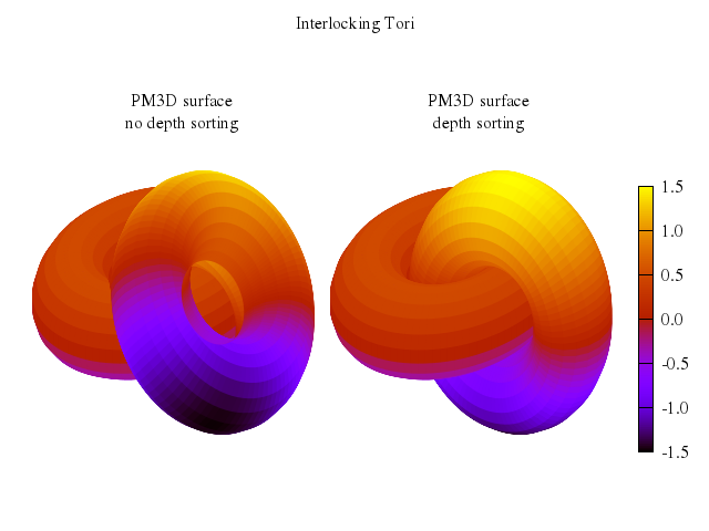
## 3D mapping
[Original Demo](http://gnuplot.sourceforge.net/demo_4.6/world2.html)
### 1
```ruby
# # Plot of location on globe,
# # this time with labels color-coded by explicit 4th input column
# # Requires EAM_DATASTRINGS
# #
# set dummy u,v
# set angles degrees
# set parametric
# set view 60, 136, 1.22, 1.26
# set samples 64,64
# set isosamples 13,13
# set mapping spherical
# unset xtics
# unset ytics
# unset ztics
# set border 0
# set title "Labels colored by GeV plotted in spherical coordinate system"
# set urange [ -90.0000 : 90.0000 ] noreverse nowriteback
# set vrange [ 0.00000 : 360.000 ] noreverse nowriteback
# set cblabel "GeV"
# set cbrange [0:8]
# set colorb vert user size 0.02, 0.75
# unset hidden
# splot cos(u)*cos(v),cos(u)*sin(v),sin(u) notitle with lines lt 5, \
# 'world.dat' notitle with lines lt 2, \
# 'srl.dat' using 3:2:(1):1:4 with labels notitle point pt 6 lw .1 left offset 1,0 font "Helvetica,7" tc pal
Numo.gnuplot do
set dummy:"u,v"
set angles:"degrees"
set :parametric
set view:[60,136,1.22,1.26]
set samples:[64,64]
set isosamples:[13,13]
set mapping:"spherical"
unset :xtics
unset :ytics
unset :ztics
set border:0
set title:"Labels colored by GeV plotted in spherical coordinate system"
set urange:-90.0000..90.0000, noreverse:true, nowriteback:true
set vrange:0.00000..360.000, noreverse:true, nowriteback:true
set cblabel:"GeV"
set cbrange:0..8
set :colorb, :vert, "user", size:[0.02,0.75]
unset :hidden
splot "cos(u)*cos(v)",
"cos(u)*sin(v)",
["sin(u)", :notitle, with:"lines", lt:5],
["'world.dat'", :notitle, with:"lines", lt:2],
["'srl.dat'", using:'3:2:(1):1:4', with:"labels", notitle:true, point_pt:6, lw:0.1, left:true, offset:1],
["0", font:"Helvetica,7", tc_pal:true]
end
```
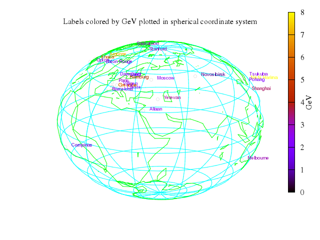
### 2
```ruby
# set title "Labels with hidden line removal"
# set hidden nooffset
# replot
Numo.gnuplot do
set title:"Labels with hidden line removal"
set :hidden, :nooffset
replot
end
```
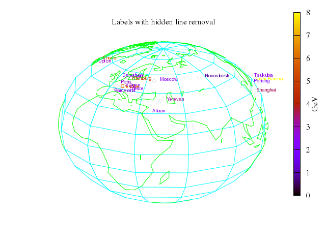
## polar coords
[Original Demo](http://gnuplot.sourceforge.net/demo_4.6/polar.html)
### 1
```ruby
# # Show some of the new polar capabilities.
# #
# unset border
# set clip
# set polar
# set xtics axis nomirror
# set ytics axis nomirror
# unset rtics
# set samples 160
# set zeroaxis
# set trange [0:2*pi]
# set title "Three circles (with aspect ratio distortion)"
# plot .5,1,1.5
Numo.gnuplot do
unset :border
set :clip
set :polar
set :xtics, :axis, :nomirror
set :ytics, :axis, :nomirror
unset :rtics
set samples:160
set :zeroaxis
set trange:"[0:2*pi]"
set title:"Three circles (with aspect ratio distortion)"
plot ".5",
"1",
"1.5"
end
```
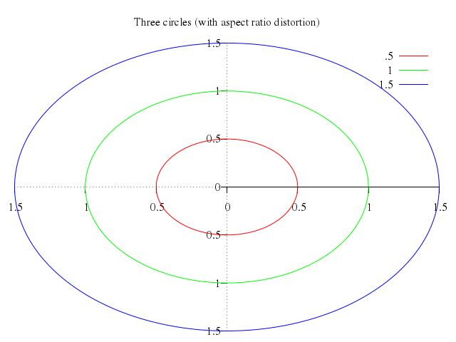
### 2
```ruby
# set title ""
# set key box
#
# plot cos(2*t)
Numo.gnuplot do
set title:""
set :key, :box
plot "cos(2*t)"
end
```
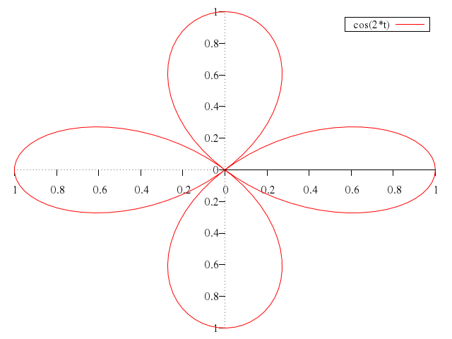
### 3
```ruby
# plot 2*sqrt(cos(t)),-2*sqrt(cos(t))
Numo.gnuplot do
plot "2*sqrt(cos(t))",
"-2*sqrt(cos(t))"
end
```
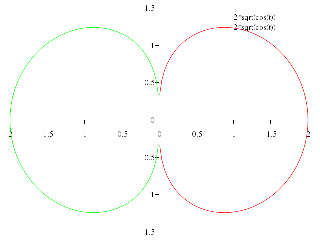
### 4
```ruby
# plot sin(4*t),cos(4*t)
Numo.gnuplot do
plot "sin(4*t)",
"cos(4*t)"
end
```
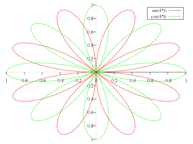
### 5
```ruby
# set offset 0,0,0,0
#
# set xrange [-5:5]
# set yrange [-5:5]
# plot t/cos(3*t)
Numo.gnuplot do
set offset:[0,0,0,0]
set xrange:-5..5
set yrange:-5..5
plot "t/cos(3*t)"
end
```
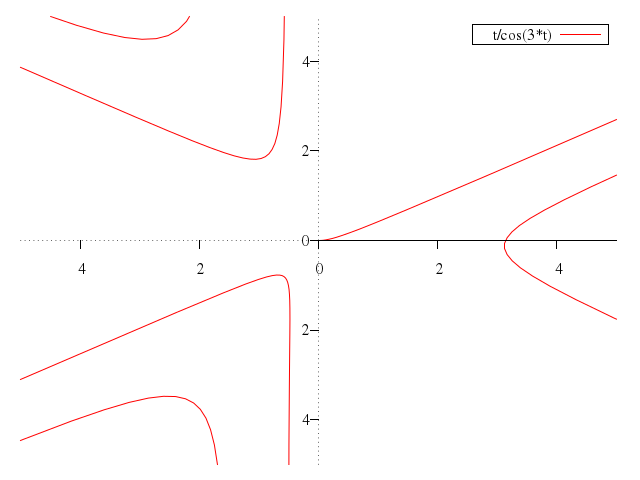
### 6
```ruby
# set autoscale
#
# plot 1-sin(t)
Numo.gnuplot do
set :autoscale
plot "1-sin(t)"
end
```
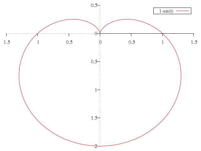
### 7
```ruby
# set trange [0:12*pi]
# plot 2*t
Numo.gnuplot do
set trange:"[0:12*pi]"
plot "2*t"
end
```
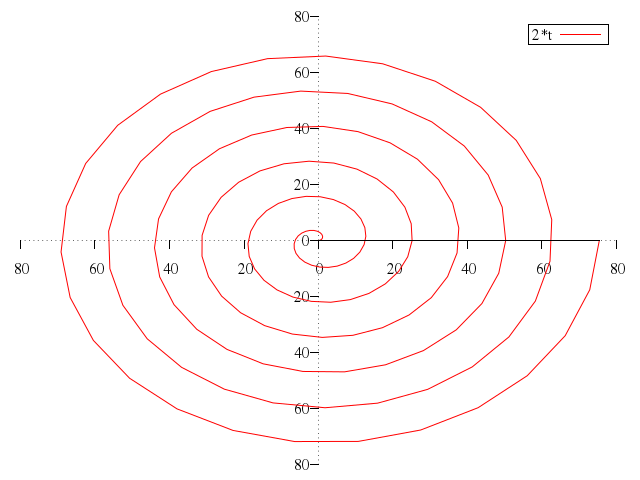
### 8
```ruby
# butterfly(x)=exp(cos(x))-2*cos(4*x)+sin(x/12)**5
# set samples 800
# set title "Butterfly"
# unset key
# plot butterfly(t)
Numo.gnuplot do
run "butterfly(x)=exp(cos(x))-2*cos(4*x)+sin(x/12)**5"
set samples:800
set title:"Butterfly"
unset :key
plot "butterfly(t)"
end
```
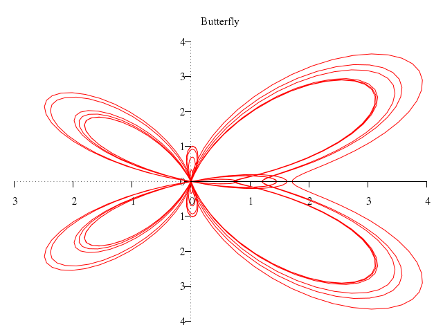
### 9
```ruby
# reset
#
# set polar
# set grid polar
# unset xtics
# unset ytics
# set border 0
# set style fill solid 0.5
# set rrange [0.1 : 4]
# set size square
# set key title "bounding radius 2.5"
# set key outside top right samplen 0.7
#
# plot 3.+sin(t)*cos(5*t) with filledcurve above r=2.5 notitle,\
# 3.+sin(t)*cos(5*t) with line
Numo.gnuplot do
reset
set :polar
set :grid, :polar
unset :xtics
unset :ytics
set border:0
set :style, fill_solid:0.5
set rrange:0.1..4
set size:"square"
set :key, title:"bounding radius 2.5"
set :key, :outside, :top, :right, samplen:0.7
plot ["3.+sin(t)*cos(5*t)", with:'filledcurve above r=2.5', notitle:true],
["3.+sin(t)*cos(5*t)", with:"line"]
end
```
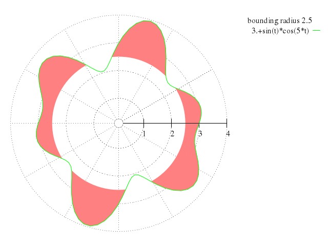
## polar data
[Original Demo](http://gnuplot.sourceforge.net/demo_4.6/poldat.html)
### 1
```ruby
# set size square
# set time
# set clip
# set xtics axis nomirror
# set ytics axis nomirror
# unset grid
# unset polar
# set title "Primitive Smith Chart"
# unset key
# set xlabel "Impedance or Admittance Coordinates"
# set para
# set rrange [-0 : 10]
# set trange [-pi : pi]
# set xrange [-1:1]
# set yrange [-1:1]
# tv(t,r) = sin(t)/(1+r)
# tu(t,r) = (cos(t) +r)/(1+r)
# cu(t,x) = 1 + cos(t)/x
# cv(t,x) = (1+ sin(t))/x
# plot cu(t,.1),cv(t,.1),cu(t,.1),-cv(t,.1),\
# cu(t,1),cv(t,1),cu(t,1),-cv(t,1),\
# cu(t,10),cv(t,10),cu(t,10),-cv(t,10),\
# tu(t,.1),tv(t,.1),\
# tu(t,.5),tv(t,.5),\
# tu(t,1),tv(t,1),\
# tu(t,5),tv(t,5),\
# tu(t,10),tv(t,10),\
# cu(t,.5),cv(t,.5),cu(t,.5),-cv(t,.5),\
# tu(t,0),tv(t,0)
Numo.gnuplot do
set size:"square"
#set :time
set :clip
set :xtics, :axis, :nomirror
set :ytics, :axis, :nomirror
unset :grid
unset :polar
set title:"Primitive Smith Chart"
unset :key
set xlabel:"Impedance or Admittance Coordinates"
set :para
set rrange:-0..10
set trange:"[-pi:pi]"
set xrange:-1..1
set yrange:-1..1
run "tv(t,r) = sin(t)/(1+r)"
run "tu(t,r) = (cos(t) +r)/(1+r)"
run "cu(t,x) = 1 + cos(t)/x"
run "cv(t,x) = (1+ sin(t))/x"
plot "cu(t,.1)",
"cv(t,.1)",
"cu(t,.1)",
"-cv(t,.1)",
"cu(t,1)",
"cv(t,1)",
"cu(t,1)",
"-cv(t,1)",
"cu(t,10)",
"cv(t,10)",
"cu(t,10)",
"-cv(t,10)",
"tu(t,.1)",
"tv(t,.1)",
"tu(t,.5)",
"tv(t,.5)",
"tu(t,1)",
"tv(t,1)",
"tu(t,5)",
"tv(t,5)",
"tu(t,10)",
"tv(t,10)",
"cu(t,.5)",
"cv(t,.5)",
"cu(t,.5)",
"-cv(t,.5)",
"tu(t,0)",
"tv(t,0)"
end
```
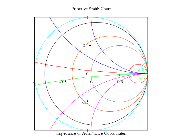
### 2
```ruby
# #cu(t,5),cv(t,5),cu(t,5),-cv(t,5)
# set angles degrees
# set polar
# set grid polar 15.
# unset border
# unset param
# set title "Antenna Pattern"
# set xlabel "Azimuth"
# set ylabel "dBSM"
# set style data line
# set rrange [-200:60]
# set trange [-pi:pi]
# set xrange [-220:220]
# set yrange [-220:220]
# unset xtics
# plot "-" using 1:5,"-"
# # Input data ncmain.d4 generated by genpat2.f:Tx antenna pattern
# # x,y,z of center point B in coord 3
# # -5.12 0 -1.5
# # euler matrix
# # 0 -1 0
# # 0.7071 0 0.7071
# # -0.7071 0 0.7071
# # theta(deg) phi(deg) E-theta(dB) phase E-phi(dB) phase
# 0 0 -200 0 18.992 0
# 2 0 -200 0 18.898 0
# 4 0 -200 0 18.619 0
# 6 0 -200 0 18.152 0
# 8 0 -200 0 17.497 0
# 10 0 -200 0 16.651 0
# 12 0 -200 0 15.614 0
# 14 0 -200 0 14.382 0
# 16 0 -200 0 12.952 0
# 18 0 -200 0 11.32 0
# 20 0 -200 0 9.483 0
# 22 0 -200 0 7.434 0
# 24 0 -200 0 5.169 0
# 26 0 -200 0 2.68 0
# 28 0 -200 0 -0.039 0
# 30 0 -200 0 -2.998 0
# 32 0 -200 0 -6.204 0
# 34 0 -200 0 -9.67 0
# 36 0 -200 0 -13.407 0
# 38 0 -200 0 -17.429 0
# 40 0 -200 0 -21.751 0
# 42 0 -200 0 -26.391 0
# 44 0 -200 0 -31.368 0
# 46 0 -200 0 -36.705 0
# 48 0 -200 0 -42.429 0
# 50 0 -200 0 -48.569 0
# 52 0 -200 0 -55.16 0
# 54 0 -200 0 -62.243 0
# 56 0 -200 0 -69.867 0
# 58 0 -200 0 -78.087 0
# 60 0 -200 0 -86.971 0
# 62 0 -200 0 -96.602 0
# 64 0 -200 0 -107.08 0
# 66 0 -200 0 -118.53 0
# 68 0 -200 0 -131.11 0
# 70 0 -200 0 -145.022 0
# 72 0 -200 0 -160.534 0
# 74 0 -200 0 -177.982 0
# 76 0 -200 0 -195.848 0
# 78 0 -200 0 -199.967 0
# 80 0 -200 0 -200 0
# 82 0 -200 0 -200 0
# 84 0 -200 0 -200 0
# 86 0 -200 0 -200 0
# 88 0 -200 0 -200 0
# 90 0 -200 0 -200 0
# 92 0 -200 0 -200 0
# 94 0 -200 0 -200 0
# 96 0 -200 0 -200 0
# 98 0 -200 0 -200 0
# 100 0 -200 0 -200 0
# 102 0 -200 0 -200 0
# 104 0 -200 0 -200 0
# 106 0 -200 0 -200 0
# 108 0 -200 0 -200 0
# 110 0 -200 0 -200 0
# 112 0 -200 0 -200 0
# 114 0 -200 0 -200 0
# 116 0 -200 0 -200 0
# 118 0 -200 0 -200 0
# 120 0 -200 0 -200 0
# 122 0 -200 0 -200 0
# 124 0 -200 0 -200 0
# 126 0 -200 0 -200 0
# 128 0 -200 0 -200 0
# 130 0 -200 0 -200 0
# 132 0 -200 0 -200 0
# 134 0 -200 0 -200 0
# 136 0 -200 0 -200 0
# 138 0 -200 0 -200 0
# 140 0 -200 0 -200 0
# 142 0 -200 0 -200 0
# 144 0 -200 0 -200 0
# 146 0 -200 0 -200 0
# 148 0 -200 0 -200 0
# 150 0 -200 0 -200 0
# 152 0 -200 0 -200 0
# 154 0 -200 0 -200 0
# 156 0 -200 0 -200 0
# 158 0 -200 0 -200 0
# 160 0 -200 0 -200 0
# 162 0 -200 0 -200 0
# 164 0 -200 0 -200 0
# 166 0 -200 0 -200 0
# 168 0 -200 0 -200 0
# 170 0 -200 0 -200 0
# 172 0 -200 0 -200 0
# 174 0 -200 0 -200 0
# 176 0 -200 0 -200 0
# 178 0 -200 0 -200 0
# 180 0 -200 0 -200 0
# e
# 0 9.0007 -35.926 -71.297 9.0783
# 2 8.1667 0.13355 -32.735 8.9007
# 4 6.0696 4.0782 -28.04 8.3501
# 6 3.3053 4.8742 -26.062 7.3795
# 8 0.131 4.2554 -25.105 5.9101
# 10 -3.4589 2.6769 -24.794 3.8084
# 12 -7.6407 0.15917 -25.211 0.82257
# 14 -12.849 -3.6543 -26.702 -3.6253
# 16 -20.405 -10.185 -30.112 -11.564
# 18 -41.802 -37.181 -39.114 -24.83
# 20 -25.979 -11.868 -38.677 -10.86
# 22 -22.06 -7.1064 -29.743 -7.4312
# 24 -21.258 -5.2193 -26.432 -6.2183
# 26 -22.103 -4.8803 -25.429 -5.9416
# 28 -24.356 -5.858 -26.299 -6.0712
# 30 -28.216 -8.3757 -29.576 -6.4985
# 32 -33.989 -13.34 -38.93 -7.5039
# 34 -37.632 -21.69 -37.458 -9.6424
# 36 -35.691 -16.286 -29.566 -13.578
# 38 -35.22 -12.594 -27.052 -15.787
# 40 -36.549 -12.197 -27.142 -11.075
# 42 -38.418 -14.735 -29.897 -7.6375
# 44 -39.287 -23.397 -38.646 -6.0943
# 46 -39.287 -23.397 -38.646 -6.0943
# 48 -38.418 -14.735 -29.897 -7.6375
# 50 -36.549 -12.197 -27.142 -11.075
# 52 -35.22 -12.594 -27.052 -15.787
# 54 -35.691 -16.286 -29.566 -13.578
# 56 -37.632 -21.69 -37.458 -9.6424
# 58 -33.989 -13.34 -38.93 -7.5039
# 60 -28.216 -8.3757 -29.576 -6.4985
# 62 -24.356 -5.858 -26.299 -6.0712
# 64 -22.103 -4.8803 -25.429 -5.9416
# 66 -21.258 -5.2193 -26.432 -6.2183
# 68 -22.06 -7.1064 -29.743 -7.4312
# 70 -25.979 -11.868 -38.677 -10.86
# 72 -41.802 -37.18 -39.114 -24.83
# 74 -20.405 -10.185 -30.112 -11.564
# 76 -12.849 -3.6543 -26.702 -3.6253
# 78 -7.6407 0.15917 -25.211 0.82257
# 80 -3.4589 2.6769 -24.794 3.8084
# 82 0.131 4.2554 -25.105 5.9101
# 84 3.3053 4.8742 -26.062 7.3795
# 86 6.0696 4.0782 -28.04 8.3501
# 88 8.1667 0.13355 -32.735 8.9007
# 90 9.0007 -35.926 -71.297 9.0783
# 92 8.1667 0.13355 -32.735 8.9007
# 94 6.0696 4.0782 -28.04 8.3501
# 96 3.3053 4.8742 -26.062 7.3795
# 98 0.131 4.2554 -25.105 5.9101
# 100 -3.4589 2.6769 -24.794 3.8084
# 102 -7.6407 0.15917 -25.211 0.82257
# 104 -12.849 -3.6543 -26.702 -3.6253
# 106 -20.405 -10.185 -30.112 -11.564
# 108 -41.802 -37.181 -39.114 -24.83
# 110 -25.979 -11.868 -38.677 -10.86
# 112 -22.06 -7.1064 -29.743 -7.4312
# 114 -21.258 -5.2193 -26.432 -6.2183
# 116 -22.103 -4.8803 -25.429 -5.9416
# 118 -24.356 -5.858 -26.299 -6.0712
# 120 -28.216 -8.3757 -29.576 -6.4985
# 122 -33.989 -13.34 -38.93 -7.5039
# 124 -37.632 -21.69 -37.458 -9.6424
# 126 -35.691 -16.286 -29.566 -13.578
# 128 -35.22 -12.594 -27.052 -15.787
# 130 -36.549 -12.197 -27.142 -11.075
# 132 -38.418 -14.735 -29.897 -7.6375
# 134 -39.287 -23.397 -38.646 -6.0943
# 136 -39.287 -23.397 -38.646 -6.0943
# 138 -38.418 -14.735 -29.897 -7.6375
# 140 -36.549 -12.197 -27.142 -11.075
# 142 -35.22 -12.594 -27.052 -15.787
# 144 -35.691 -16.286 -29.566 -13.578
# 146 -37.632 -21.69 -37.458 -9.6424
# 148 -33.989 -13.34 -38.93 -7.5039
# 150 -28.216 -8.3757 -29.576 -6.4985
# 152 -24.356 -5.858 -26.299 -6.0712
# 154 -22.103 -4.8803 -25.429 -5.9416
# 156 -21.258 -5.2193 -26.432 -6.2183
# 158 -22.06 -7.1064 -29.743 -7.4312
# 160 -25.979 -11.868 -38.677 -10.86
# 162 -41.802 -37.181 -39.114 -24.83
# 164 -20.405 -10.185 -30.112 -11.564
# 166 -12.849 -3.6543 -26.702 -3.6253
# 168 -7.6407 0.15917 -25.211 0.82257
# 170 -3.4589 2.6769 -24.794 3.8084
# 172 0.131 4.2554 -25.105 5.9101
# 174 3.3053 4.8742 -26.062 7.3795
# 176 6.0696 4.0782 -28.04 8.3501
# 178 8.1667 0.13355 -32.735 8.9007
# 180 9.0007 -35.926 -71.297 9.0783
# 182 8.1667 0.13355 -32.735 8.9007
# 184 6.0696 4.0782 -28.04 8.3501
# 186 3.3053 4.8742 -26.062 7.3795
# 188 0.131 4.2554 -25.105 5.9101
# 190 -3.4589 2.6769 -24.794 3.8084
# 192 -7.6407 0.15917 -25.211 0.82257
# 194 -12.849 -3.6543 -26.702 -3.6253
# 196 -20.405 -10.185 -30.112 -11.564
# 198 -41.802 -37.181 -39.114 -24.83
# 200 -25.979 -11.868 -38.677 -10.86
# 202 -22.06 -7.1064 -29.743 -7.4312
# 204 -21.258 -5.2193 -26.432 -6.2183
# 206 -22.103 -4.8803 -25.429 -5.9416
# 208 -24.356 -5.858 -26.299 -6.0712
# 210 -28.216 -8.3757 -29.576 -6.4985
# 212 -33.989 -13.34 -38.93 -7.5039
# 214 -37.632 -21.69 -37.458 -9.6424
# 216 -35.691 -16.286 -29.566 -13.578
# 218 -35.22 -12.594 -27.052 -15.787
# 220 -36.549 -12.197 -27.142 -11.075
# 222 -38.418 -14.735 -29.897 -7.6375
# 224 -39.287 -23.397 -38.646 -6.0943
# 226 -39.287 -23.397 -38.646 -6.0943
# 228 -38.418 -14.735 -29.897 -7.6375
# 230 -36.549 -12.197 -27.142 -11.075
# 232 -35.22 -12.594 -27.052 -15.787
# 234 -35.691 -16.286 -29.566 -13.578
# 236 -37.632 -21.69 -37.458 -9.6424
# 238 -33.989 -13.34 -38.93 -7.5039
# 240 -28.216 -8.3757 -29.576 -6.4985
# 242 -24.356 -5.858 -26.299 -6.0712
# 244 -22.103 -4.8803 -25.429 -5.9416
# 246 -21.258 -5.2193 -26.432 -6.2183
# 248 -22.06 -7.1064 -29.743 -7.4312
# 250 -25.979 -11.868 -38.677 -10.86
# 252 -41.802 -37.18 -39.114 -24.83
# 254 -20.405 -10.185 -30.112 -11.564
# 256 -12.849 -3.6543 -26.702 -3.6253
# 258 -7.6407 0.15917 -25.211 0.82257
# 260 -3.4589 2.6769 -24.794 3.8084
# 262 0.131 4.2554 -25.105 5.9101
# 264 3.3053 4.8742 -26.062 7.3795
# 266 6.0696 4.0782 -28.04 8.3501
# 268 8.1667 0.13355 -32.735 8.9007
# 270 9.0007 -35.926 -71.297 9.0783
# 272 8.1667 0.13355 -32.735 8.9007
# 274 6.0696 4.0782 -28.04 8.3501
# 276 3.3053 4.8742 -26.062 7.3795
# 278 0.13099 4.2554 -25.105 5.9101
# 280 -3.4589 2.6769 -24.794 3.8084
# 282 -7.6407 0.15917 -25.211 0.82257
# 284 -12.849 -3.6543 -26.702 -3.6253
# 286 -20.405 -10.185 -30.112 -11.564
# 288 -41.802 -37.181 -39.114 -24.83
# 290 -25.979 -11.868 -38.677 -10.86
# 292 -22.06 -7.1064 -29.743 -7.4312
# 294 -21.258 -5.2193 -26.432 -6.2183
# 296 -22.103 -4.8803 -25.429 -5.9416
# 298 -24.356 -5.858 -26.299 -6.0712
# 300 -28.216 -8.3757 -29.576 -6.4985
# 302 -33.989 -13.34 -38.93 -7.5039
# 304 -37.632 -21.69 -37.458 -9.6424
# 306 -35.691 -16.286 -29.566 -13.578
# 308 -35.22 -12.594 -27.052 -15.787
# 310 -36.549 -12.197 -27.142 -11.075
# 312 -38.418 -14.735 -29.897 -7.6375
# 314 -39.287 -23.397 -38.646 -6.0943
# 316 -39.287 -23.397 -38.646 -6.0943
# 318 -38.418 -14.735 -29.897 -7.6375
# 320 -36.549 -12.197 -27.142 -11.075
# 322 -35.22 -12.594 -27.052 -15.787
# 324 -35.691 -16.286 -29.566 -13.578
# 326 -37.632 -21.69 -37.458 -9.6424
# 328 -33.989 -13.34 -38.93 -7.5039
# 330 -28.216 -8.3757 -29.576 -6.4985
# 332 -24.356 -5.858 -26.299 -6.0712
# 334 -22.103 -4.8803 -25.429 -5.9416
# 336 -21.258 -5.2193 -26.432 -6.2183
# 338 -22.06 -7.1064 -29.743 -7.4312
# 340 -25.979 -11.868 -38.677 -10.86
# 342 -41.802 -37.181 -39.114 -24.83
# 344 -20.405 -10.185 -30.112 -11.564
# 346 -12.849 -3.6543 -26.702 -3.6253
# 348 -7.6407 0.15917 -25.211 0.82257
# 350 -3.4589 2.6769 -24.794 3.8084
# 352 0.131 4.2554 -25.105 5.9101
# 354 3.3053 4.8742 -26.062 7.3795
# 356 6.0696 4.0782 -28.04 8.3501
# 358 8.1667 0.13355 -32.735 8.9007
# 360 9.0007 -35.926 -71.297 9.0783
# e
#
# reset
Numo.gnuplot do
set angles:"degrees"
set :polar
set :grid, :polar, 15.0
unset :border
unset :param
set title:"Antenna Pattern"
set xlabel:"Azimuth"
set ylabel:"dBSM"
set :style, :data, :line
set rrange:-200..60
set trange:"[-pi:pi]"
set xrange:-220..220
set yrange:-220..220
unset :xtics
run <>> Skipping demo <<<\n" ; \
# print "This copy of gnuplot was built without support for plotting images" ; \
# exit ;
#
# print ""
# print "The plotting styles \`image\` and \`rgbimage\` are intended for plotting"
# print "images described in a data file either in the convential ASCII format or"
# print "in a binary format described by the qualifiers \`binary\` and \`using\`."
# print "All pixels have an (x,y) or (x,y,z) coordinate. These values can be"
# print "included in the data file or implicitly determined with the sampling"
# print "\'array\' key word and sampling periods \'dx\' and \'dy\'. The key words"
# print "\'rotate\' and, for 3d plots, \'perpendicular\' control orientation."
# print "\nThe data for this image was stored as RGB triples, one byte per channel,"
# print "without (x,y) coordinate information. This yields a most compact file."
# print "The plotting command is displayed on the graph."
# print ""
# reset
# set title "Larry Ewing's GIMP penguin on vacation basking in\nthe balmy waters off the coast of Murmansk"
# set xrange [-10:137]
# set yrange [-10:157]
# set label "\"I flew here... by plane. Why? For the halibut.\"" at 64,135 center
# plot 'blutux.rgb' binary array=(128,128) flipy format='%uchar' with rgbimage
Numo.gnuplot do
reset
set title:"Larry Ewing's GIMP penguin on vacation basking in\nthe balmy waters off the coast of Murmansk"
set xrange:-10..137
set yrange:-10..157
set label:"\"I flew here... by plane. Why? For the halibut.\"", at:[64,135], center:true
plot "'blutux.rgb'", binary:'array=(128,128) flipy format="%uchar"', with:"rgbimage"
end
```
### 2
```ruby
# reset
#
# print ""
# print "Images are typically stored in a file with the first datum being the"
# print "top, left pixel. Without the ability to translate coordinates, the"
# print "the result would be an upside down image."
# print ""
# print "The key word \'array\' means an implied sample array is applied"
# print "to generate the locations of file data using the sampling periods"
# print "dx, dy and dz. The x-dimension is always the contiguous points in"
# print "a binary file. The y-dimension is the line number which is incremented"
# print "upon the x-dimension reaching the line length. The z-dimension is"
# print "the plane number which is incremented upon the y-dimension reaching"
# print "the number of lines per plane."
# print ""
# print "To alter the location of the binary data when displayed via the \'plot\'"
# print "command, use the key word \'rotate\' along with changing the sign of dx, dy"
# print "and dz."
# print ""
# set title "Translations of position variables via 'using'"
# set xrange [-10:275]
# set yrange [-10:300]
# unset key
# set label "\"Time for a dip...\"" at 132,285 center
# plot 'blutux.rgb' binary array=(128,128) flipy center=( 64,201 ) format='%uchar' with rgbimage, \
# 'blutux.rgb' binary array=(128,128) flipy rotation=-90d center=(201,201) format='%uchar' with rgbimage, \
# 'blutux.rgb' binary array=(128,128) flip=y rotate=3.1415 center=(201,64) format='%uchar' with rgbimage, \
# 'blutux.rgb' binary array=(128,128) flip=y rot=0.5pi center=(64,64) format='%uchar' using 1:2:3 with rgbimage
Numo.gnuplot do
reset
set title:"Translations of position variables via 'using'"
set xrange:-10..275
set yrange:-10..300
unset :key
set label:"\"Time for a dip...\"", at:[132,285], center:true
plot ["'blutux.rgb'", binary:'array=(128,128) flipy center=( 64,201 ) format="%uchar"', with:"rgbimage"],
["'blutux.rgb'", binary:'array=(128,128) flipy rotation=-90d center=(201,201) format="%uchar"', with:"rgbimage"],
["'blutux.rgb'", binary:'array=(128,128) flip=y rotate=3.1415 center=(201,64) format="%uchar"', with:"rgbimage"],
["'blutux.rgb'", binary:'array=(128,128) flip=y rot=0.5pi center=(64,64) format="%uchar"', using:[1,2,3], with:"rgbimage"]
end
```
### 3
```ruby
# reset
#
# print ""
# print "There is the ability to plot both color images and palette based"
# print "images. This is controlled by the styles \`image\`, which derives"
# print "color information from the current palette, and \`rgbimage\`,"
# print "which requires three components representing the red, blue and"
# print "green primary color scheme."
# print ""
# print "By the way, if you have a mouse active, click the right button"
# print "inside the image to isolate a portion of the image and see what"
# print "happens."
# print ""
# unset key
# set xrange [-10:137]
# set yrange [-10:157]
# set label 1 "\"I am the penguin, GOO GOO GOO JOOB.\"" at 63,140 center
# set title "Palette mode 'image' used to produce psychedelic bird"
# unset colorbox
# plot 'blutux.rgb' binary array=(128,128) flipy format='%uchar%uchar%uchar' using ($1+$2+$3) with image
Numo.gnuplot do
reset
unset :key
set xrange:-10..137
set yrange:-10..157
set :label, 1, "\"I am the penguin, GOO GOO GOO JOOB.\"", at:[63,140], center:true
set title:"Palette mode 'image' used to produce psychedelic bird"
unset :colorbox
plot "'blutux.rgb'", binary:'array=(128,128) flipy format="%uchar%uchar%uchar"', using:'($1+$2+$3)', with:"image"
end
```
### 4
```ruby
# reset
#
# print ""
# print "Naturally, as with 3d color surfaces, the palette may be changed."
# print "This is an example of gray scale."
# print ""
# print "Also, notice in the plot command the key word \'flipy\'. This"
# print "means to change the direction of the sample along the y dimension"
# print "and is useful for the situation where images or other data are"
# print "stored in some direction other than that of the Cartesion system."
# print "Alone, \'flipD\' means do flipping in the D (x y or z) direction"
# print "for all records. Individual records can be controlled using the"
# print "syntax \'flipD=#,...,#\', where # is \'0\' or \'1\'."
# print ""
# unset key
# set xrange [-10:137]
# set yrange [-10:157]
# set tics out
# set label 1 "\"This picture was taken by my friend Ansel Adams.\"" at 63,140 center
# set title "The palette can be changed from color to gray scale"
# set palette gray
# unset colorbox
# plot 'blutux.rgb' binary array=(128,128) flipy format='%uchar%uchar%uchar' using ($1+$2+$3)/3 with image
Numo.gnuplot do
reset
unset :key
set xrange:-10..137
set yrange:-10..157
set :tics, :out
set :label, 1, "\"This picture was taken by my friend Ansel Adams.\"", at:[63,140], center:true
set title:"The palette can be changed from color to gray scale"
set :palette, "gray"
unset :colorbox
plot "'blutux.rgb'", binary:'array=(128,128) flipy format="%uchar%uchar%uchar"', using:'($1+$2+$3)/3', with:"image"
end
```
### 5
```ruby
# unset label 1
#
# print ""
# print "Also, similar to 3d color surface plots, a color box showing the"
# print "palette mapping scheme can be added to the plot. The default"
# print "location is the right edge of the plot. The location can be set"
# print "manually using \`set colorbox\` and \`set margin\`."
# print ""
# print "As a prelude to the next graph, resize the plot window to judge"
# print "the refresh speed of the image drawing routine. Notice that when"
# print "the window is smaller, the image refresh is faster. There is more"
# print "decimation in the data of the original image and less data to plot."
# print "Furthermore, the window continues to refresh at a reasonable rate"
# print "even when the input image size becomes large (e.g., 1024 x 1024)"
# print "because the number of pixels on the screen remains about the same"
# print "while much of the hi resolution data is decimated."
# print ""
# unset key
# set pm3d map
# set xrange [10:117]
# set yrange [10:117]
# set tics out
# set colorbox
# set cbrange [0:255]
# set title "As with 3d color surfaces, a color box may be added to the plot"
# splot 'blutux.rgb' binary array=(128,128) flipy format='%uchar%uchar%uchar' using ($1+$2+$3)/3 with image
Numo.gnuplot do
unset label:1
unset :key
set :pm3d, :map
set xrange:10..117
set yrange:10..117
set :tics, :out
set :colorbox
set cbrange:0..255
set title:"As with 3d color surfaces, a color box may be added to the plot"
splot "'blutux.rgb'", binary:'array=(128,128) flipy format="%uchar%uchar%uchar"', using:'($1+$2+$3)/3', with:"image"
end
```
### 6
```ruby
# print ""
# print "The \'rotation\' key word works not only with angles of integer"
# print "multiples of 90 degrees but also arbitrary rotations. When"
# print "constructing an image, Gnuplot verifies that pixel locations"
# print "form a valid grid. Pixel widths are based upon the grid"
# print "spacing. If the image orientation is aligned with the view"
# print "axes, Gnuplot uses an efficient image driver routine. Otherwise,"
# print "individual pixels are drawn using polygon shapes."
# print ""
# print "Resize this window and compare the plot's refresh rate to that of"
# print "the previous and next plot. Notice how in this example if the"
# print "window is small the image refresh does not speed up. Unlike the"
# print "image routine where image data is decimated, all color rectangles"
# print "must be redrawn no matter the size of the output image."
# print ""
# print "Also notice how the center of the image matches the tuple specified"
# print "with the key word \'center\' in the plot command. Before doing the"
# print "rotation, the image's natural center is subtracted, and after doing"
# print "the rotation, the specified center is added."
# print ""
# set key
# set xrange [-10:138]
# set yrange [-10:138]
# set tics out
# set title "Polygons used to draw pixels for rotated images\nNotice the slower refresh rate than for the next plot"
# unset colorbox
# plot 'blutux.rgb' binary array=(128,128) dx=0.70711 dy=0.70711 flipy rotation=45d center=(63.5,63.5) format='%uchar' using ($1+$2+$3)/3 with image
Numo.gnuplot do
set :key
set xrange:-10..138
set yrange:-10..138
set :tics, :out
set title:"Polygons used to draw pixels for rotated images\nNotice the slower refresh rate than for the next plot"
unset :colorbox
plot "'blutux.rgb'", binary:'array=(128,128) dx=0.70711 dy=0.70711 flipy rotation=45d center=(63.5,63.5) format="%uchar"', using:'($1+$2+$3)/3', with:"image"
end
```
### 7
```ruby
# reset
#
# print ""
# print "The image of this plot is rotated 90 degrees and can utilize the"
# print "efficient image functions of terminal drivers. The plot refresh"
# print "is faster than the previous plot."
# print ""
# print "Furthermore, the image location in this case is specified via the"
# print "\'origin\' key word. As such, the rotation is done about the origin"
# print "as opposed to the center of the image. Notice the difference in"
# print "axis ranges."
# print ""
# unset key
# set xrange [-138:10]
# set yrange [-10:138]
# set tics out
# set title "Terminal image routine used to draw plot rotated about origin\nNotice the faster refresh rate than for the previous plot"
# unset colorbox
# plot 'blutux.rgb' binary array=(128,128) dx=1 flip=y rotation=0.5pi origin=(0,0) format='%uchar' using ($1+$2+$3)/3 with image
Numo.gnuplot do
reset
unset :key
set xrange:-138..10
set yrange:-10..138
set :tics, :out
set title:"Terminal image routine used to draw plot rotated about origin\nNotice the faster refresh rate than for the previous plot"
unset :colorbox
plot "'blutux.rgb'", binary:'array=(128,128) dx=1 flip=y rotation=0.5pi origin=(0,0) format="%uchar"', using:'($1+$2+$3)/3', with:"image"
end
```
### 8
```ruby
# reset
#
# print ""
# print "Algebraic manipulation of the input variables can select various"
# print "components of the image. Here are three examples where two"
# print "channels--or analogous to the ASCII file, data \"columns\"--are ignored"
# print "This is done by using \`*\` in the format to indicate that a variable"
# print "of a certain size should be discarded. For example, to select the"
# print "green channel, \`%*uchar%uchar%*uchar\` is one alternative."
# print ""
# set size 1.0, 1.0
# set origin 0.0, 0.0
# set multiplot
# set size 0.5,0.48
# set origin 0.0,0.47
# unset key
# set xrange [-0.5:127.5]
# set yrange [-0.5:127.5]
# set tics out
# set label 1 "Selection of the input channels via \`using\`" at 140,160 center
# set title '"I do impersonations..."' offset 0,-0.5
# plot 'blutux.rgb' binary array=(128,128) flip=y format='%uchar' using 1:2:3 with rgbimage
# unset label 1
# set size 0.5,0.48
# set origin 0.5,0.47
# set title '"A cardinal."'
# plot 'blutux.rgb' binary array=(128,128) flip=y format='%uchar%*uchar%*uchar' using 1:(0):(0) with rgbimage
# set size 0.5,0.48
# set origin 0.0,0.0
# set title '"A parrot."'
# plot 'blutux.rgb' binary array=(128,128) flipy format='%*uchar%uchar%*uchar' using (0):1:(0) with rgbimage
# set size 0.5,0.48
# set origin 0.5,0.0
# set title '"A bluebird."'
# plot 'blutux.rgb' binary array=(128,128) flipy format='%*uchar%*uchar%uchar' using (0):(0):1 with rgbimage
# unset multiplot
Numo.gnuplot do
reset
set size:[1.0,1.0]
set origin:[0.0,0.0]
set :multiplot
set size:[0.5,0.48]
set origin:[0.0,0.47]
unset :key
set xrange:-0.5..127.5
set yrange:-0.5..127.5
set :tics, :out
set :label, 1, "Selection of the input channels via 'using'", at:[140,160], center:true
set title:'"I do impersonations..."', offset:[0,-0.5]
plot "'blutux.rgb'", binary:'array=(128,128) flip=y format="%uchar"', using:[1,2,3], with:"rgbimage"
unset label:1
set size:[0.5,0.48]
set origin:[0.5,0.47]
set title:'"A cardinal."'
plot "'blutux.rgb'", binary:'array=(128,128) flip=y format="%uchar%*uchar%*uchar"', using:'1:(0):(0)', with:"rgbimage"
set size:[0.5,0.48]
set origin:[0.0,0.0]
set title:'"A parrot."'
plot "'blutux.rgb'", binary:'array=(128,128) flipy format="%*uchar%uchar%*uchar"', using:'(0):1:(0)', with:"rgbimage"
set size:[0.5,0.48]
set origin:[0.5,0.0]
set title:'"A bluebird."'
plot "'blutux.rgb'", binary:'array=(128,128) flipy format="%*uchar%*uchar%uchar"', using:'(0):(0):1', with:"rgbimage"
unset :multiplot
end
```
### 9
```ruby
# reset
#
# print ""
# print "The range of valid pixel values can be set via \`cbrange\`. If the"
# print "\`cbrange\` is in autoscale mode, gnuplot will set the color scale"
# print "range of RGB images to [0:255] (8 bits of color info per channel)."
# print "This is the case in the upper left image. However, the image can be"
# print "saturated by choosing a smaller range, as done in the upper right image."
# print "Expanding the colorbox range will darken the image as in the bottom examples."
# print ""
# set size 1.0, 1.0
# set origin 0.0, 0.0
# set multiplot
# set size 0.5,0.48
# set origin 0.0,0.47
# unset key
# set xrange [-0.5:127.5]
# set yrange [-0.5:127.5]
# set tics out
# set label 1 "Luminance adjustment via \`cbrange\`" at 140,160 center
# set title 'Lake Mendota, "or Wonk-sheck-ho-mik-la!"' offset 0,-0.5
# set cbrange [*:*]
# plot 'blutux.rgb' binary array=(128,128) flipy format='%uchar' using 1:2:3 with rgbimage
# unset label 1
# set size 0.5,0.48
# set origin 0.5,0.47
# set title '"Lucky I brought sunscreen."'
# set cbrange [0:200]
# plot 'blutux.rgb' binary array=(128,128) flip=y format='%uchar' using 1:2:3 with rgbimage
# set size 0.5,0.48
# set origin 0.0,0.0
# set title 'Sunset on the Terrace'
# set cbrange [0:400]
# plot 'blutux.rgb' binary array=(128,128) flip=y format='%uchar' using (1.5*$1):2:3 with rgbimage
# set size 0.5,0.48
# set origin 0.5,0.0
# set title 'Sultry evening'
# set cbrange [0:400]
# plot 'blutux.rgb' binary array=(128,128) flipy format='%uchar' using 1:2:3 with rgbimage, '-' w points pt 7 ps 6 lt -2, '-' w points pt 7 ps 0.65 lt -2
# 110 100
# e
# 10 95
# 38 120
# 82 102
# 26 82
# 93 108
# 41 99
# 123 84
# e
# unset multiplot
Numo.gnuplot do
reset
set size:[1.0,1.0]
set origin:[0.0,0.0]
set :multiplot
set size:[0.5,0.48]
set origin:[0.0,0.47]
unset :key
set xrange:-0.5..127.5
set yrange:-0.5..127.5
set :tics, :out
set :label, 1, "Luminance adjustment via 'cbrange'", at:[140,160], center:true
set title:'Lake Mendota, "or Wonk-sheck-ho-mik-la!"', offset:[0,-0.5]
set cbrange:"[*:*]"
plot "'blutux.rgb'", binary:'array=(128,128) flipy format="%uchar"', using:[1,2,3], with:"rgbimage"
unset label:1
set size:[0.5,0.48]
set origin:[0.5,0.47]
set title:'"Lucky I brought sunscreen."'
set cbrange:0..200
plot "'blutux.rgb'", binary:'array=(128,128) flip=y format="%uchar"', using:[1,2,3], with:"rgbimage"
set size:[0.5,0.48]
set origin:[0.0,0.0]
set title:'Sunset on the Terrace'
set cbrange:0..400
plot "'blutux.rgb'", binary:'array=(128,128) flip=y format="%uchar"', using:'(1.5*$1):2:3', with:"rgbimage"
set size:[0.5,0.48]
set origin:[0.5,0.0]
set title:'Sultry evening'
set cbrange:0..400
run <>> Skipping demo <<<\n" ; \
# print "This copy of gnuplot was built without support for plotting images" ; \
# exit ;
#
# # Repeat of the 'using.dem' demo, but with binary 2d data. 'using.bin' is
# # in the format int32, int8, int16/100, int8, int16/100, int16/100.
# #
# print ""
# print "Not only can the 2d binary data mode be used for image data."
# print "Here is an example that repeats the \`using.dem\` demo with the"
# print "same data, but stored in binary format of differing sizes. It"
# print "uses different format specifiers within the \'format\' string."
# print "There are machine dependent and machine independent specifiers,"
# print "display by the command \'show datafile binary datasizes\':"
# print ""
# show datafile binary datasizes
# print ""
# set title "Convex November 1-7 1989 Circadian"
# set key left box
# set xrange[-1:24]
# plot 'using.bin' binary format='%*int32%int8%*int16%int8%*int16%*int16' using 1:2 title "Logged in" with impulses,\
# 'using.bin' binary format='%*int32%int8%*int16%int8%*int16%*int16' using 1:2 title "Logged in" with points
Numo.gnuplot do
show :datafile, binary:"datasizes"
set title:"Convex November 1-7 1989 Circadian"
set :key, :left, :box
set xrange:-1..24
plot ["'using.bin'", binary:'format="%*int32%int8%*int16%int8%*int16%*int16"', using:[1,2], title:"Logged in", with:"impulses"],
["'using.bin'", binary:'format="%*int32%int8%*int16%int8%*int16%*int16"', using:[1,2], title:"Logged in", with:"points"]
end
```

### 2
```ruby
# reset
#
# print ""
# print "Again, a different format specification for \`using\` can be"
# print "used to select different \"columns\" within the file."
# print ""
# set xrange [1:8]
# set title "Convex November 1-7 1989"
# set key below
# set label "(Weekend)" at 5,25 center
# plot 'using.bin' binary format='%*int32%*int8%int16%int8%*int16%*int16' using ($1/100):2 title "Logged in" with impulses,\
# 'using.bin' binary format='%*int32%*int8%int16%*int8%int16%*int16' using ($1/100):($2/100) t "Load average" with points,\
# 'using.bin' binary format='%*int32%*int8%int16%*int8%*int16%int16' using ($1/100):($2/100) t "%CPU used" with lines
Numo.gnuplot do
reset
set xrange:1..8
set title:"Convex November 1-7 1989"
set :key, "below"
set label:"(Weekend)", at:[5,25], center:true
plot ["'using.bin'", binary:'format="%*int32%*int8%int16%int8%*int16%*int16"', using:'($1/100):2', title:"Logged in", with:"impulses"],
["'using.bin'", binary:'format="%*int32%*int8%int16%*int8%int16%*int16"', using:'($1/100):($2/100)', t:"Load average", with:"points"],
["'using.bin'", binary:'format="%*int32%*int8%int16%*int8%*int16%int16"', using:'($1/100):($2/100)', t:"%CPU used", with:"lines"]
end
```
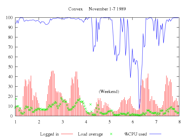
### 3
```ruby
# unset label
# reset
#
# print ""
# print "Here is another example, one repeating the \`scatter.dem\`"
# print "demo. With binary data we cannot have blank lines to"
# print "indicate a break in data, as is done with ASCII files."
# print "Instead, we can specify the record lenths in the command."
# print "In this case, the data file contains the (x,y,z) coordinate"
# print "information, hence implicit derivation of that information"
# print "is not desired. Instead, the record lengths can be specified"
# print "using the keyword \'record\', which behaves the same as"
# print "\'array\' but does not generate coordinates. The command is"
# print "displayed on the graph."
# print ""
# set title "2d binary data example where record length is part of command"
# splot 'scatter2.bin' binary endian=little record=30:30:29:26 using 1:2:3
Numo.gnuplot do
unset :label
reset
set title:"2d binary data example where record length is part of command"
splot "'scatter2.bin'", binary:'endian=little record=30:30:29:26', using:[1,2,3]
end
```
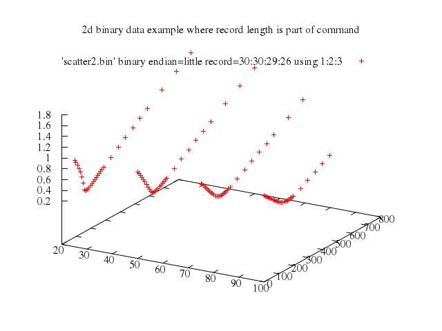
### 4
```ruby
# reset
#
# print ""
# print "For binary data, the byte endian format of the file and of the"
# print "compiler often require attention. Therefore, the key word"
# print "\'endian\' is provided for setting or interchanging byte"
# print "order. The allowable types are \'little\', \'big\', and"
# print "depending upon how your version of Gnuplot was compiled,"
# print "\'middle\' (or \'pdp\') for those still living in the medieval"
# print "age of computers. These types refer to the file's endian."
# print "Gnuplot arranges bytes according to this endian and what it"
# print "determines to be the compiler's endian."
# print ""
# print "There are also the special types \'default\' and \'swap\' (or"
# print "\'swab\') for those who don't know the file type but realize"
# print "their data looks incorrect and want to change the byte read"
# print "order."
# print ""
# print "Here is an example showing the \`scatter.dem\` data plotted"
# print "with correct and incorrect byte order. The file is known"
# print "to be little endian, so the upper left plot is correct"
# print "appearance and the upper right plot is incorrect appearance."
# print "The lower two plots are default and swapped bytes. If the"
# print "plots within the columns match, your compiler uses little"
# print "endian. If diagonal plots match then your compiler uses"
# print "big endian. If neither of the bottom plots matches the"
# print "upper plots, Tux says you're living in the past."
# print ""
# set size 1.0, 1.0
# set origin 0.0, 0.0
# set multiplot
# set size 0.5,0.48
# set origin 0.0,0.47
# unset key
# set label 1 "If plots in columns match, your compiler is little endian" at 100,1200,3.0 center
# set title 'Little endian' offset 0,-0.5
# splot 'scatter2.bin' binary record=30:30:29:26 endian=little using 1:2:3
# unset label 1
# set size 0.5,0.48
# set origin 0.5,0.47
# set title 'Big endian'
# splot 'scatter2.bin' binary record=30:30:29:26 endian=big using 1:2:3
# set size 0.5,0.48
# set origin 0.0,0.0
# set title 'Default'
# splot 'scatter2.bin' binary record=30:30:29:26 endian=default using 1:2:3
# set size 0.5,0.48
# set origin 0.5,0.0
# set title 'Swapped'
# splot 'scatter2.bin' binary record=30:30:29:26 endian=swap using 1:2:3
# unset multiplot
Numo.gnuplot do
reset
set size:[1.0,1.0]
set origin:[0.0,0.0]
set :multiplot
set size:[0.5,0.48]
set origin:[0.0,0.47]
unset :key
set :label, 1, "If plots in columns match, your compiler is little endian", at:[100,1200,3.0], center:true
set title:'Little endian', offset:[0,-0.5]
splot "'scatter2.bin'", binary:'record=30:30:29:26 endian=little', using:[1,2,3]
unset label:1
set size:[0.5,0.48]
set origin:[0.5,0.47]
set title:'Big endian'
splot "'scatter2.bin'", binary:'record=30:30:29:26 endian=big', using:[1,2,3]
set size:[0.5,0.48]
set origin:[0.0,0.0]
set title:'Default'
splot "'scatter2.bin'", binary:'record=30:30:29:26 endian=default', using:[1,2,3]
set size:[0.5,0.48]
set origin:[0.5,0.0]
set title:'Swapped'
splot "'scatter2.bin'", binary:'record=30:30:29:26 endian=swap', using:[1,2,3]
unset :multiplot
end
```
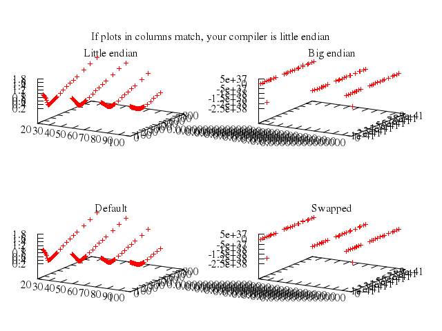
### 5
```ruby
# reset
#
# print ""
# print "This close up of a 2x2 image illustrates how pixels surround the"
# print "sampling grid points. This behavior is slightly different than"
# print "that for pm3d where the four grid points would be used to create"
# print "a single polygon element using an average, or similar mathematical"
# print "combination, of the four values at those points."
# print ""
# set title "Close up of pixels having grid points (0,0), (0,2), (2,0) and (2,2)"
# set xrange [-1.5:3.5]
# set yrange [-1.5:3.5]
# set cbrange [0:1]
# unset key
# plot '-' with rgbimage, '-' with points pt 7 ps 2 lt -1
# 0 0 0.0 0.0 0.5
# 0 2 0.0 0.5 0.0
# 2 0 0.0 0.5 0.0
# 2 2 0.0 0.0 0.5
# e
# 0 0
# 0 2
# 2 0
# 2 2
# e
# reset
Numo.gnuplot do
reset
set title:"Close up of pixels having grid points (0,0), (0,2), (2,0) and (2,2)"
set xrange:-1.5..3.5
set yrange:-1.5..3.5
set cbrange:0..1
unset :key
run < 400 ? 0 : 255
#
# plot 100.*(.4+sin(x/5.)/(x/5.)) lw 5 title 'solid line', \
# 'lena.rgb' binary array=(128,128) format="%uchar" flipy using 1:2:3:(focus(70,50)) \
# with rgbalpha title "Lena with circular mask"
Numo.gnuplot do
run "focus(x,y) = ((column(0)-x)**2 + (column(-1)-(127-y))**2) > 400 ? 0 : 255"
plot ["100.*(.4+sin(x/5.)/(x/5.))", lw:5, title:'solid line'],
["'lena.rgb'", binary:'array=(128,128) format="%uchar" flipy', using:'1:2:3:(focus(70,50))', with:"rgbalpha", title:"Lena with circular mask"]
end
```
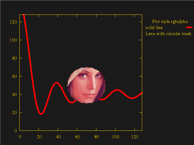
## bar chart art
[Original Demo](http://gnuplot.sourceforge.net/demo_4.6/barchart_art.html)
### 1
```ruby
# # Demo of using rescaled images to construct a bar chart
# #
# if (!strstrt(GPVAL_COMPILE_OPTIONS,"+GD_PNG")) \
# print ">>> Skipping demo <<<\n" ; \
# print "This copy of gnuplot was built without support for loading png images" ;\
# exit ;
#
# reset
# set title "Building Code Height Limits"
# unset key
#
# set xrange [ -10 : 160 ]
# set yrange [ 0 : 200 ]
# set y2range[ 0 : 200 ]
#
# set y2tics
# set grid y
#
# set xtics ("NE" 12.0, "S" 42.0, "Downtown" 72.0, "Suburbs" 127.0) scale 0.0
#
# plot 'bldg.png' binary filetype=png origin=(60,0) dx=0.5 dy=1.5 with rgbimage, \
# 'bldg.png' binary filetype=png origin=(0,0) dx=0.5 dy=1 with rgbimage, \
# 'bldg.png' binary filetype=png origin=(30,0) dx=0.5 dy=0.7 with rgbimage, \
# 'bldg.png' binary filetype=png origin=(100,0) dx=0.5 dy=0.35 with rgbimage, \
# 'bldg.png' binary filetype=png origin=(125,0) dx=0.5 dy=0.35 with rgbimage
Numo.gnuplot do
reset
set title:"Building Code Height Limits"
unset :key
set xrange:-10..160
set yrange:0..200
set y2range:0..200
set :y2tics
set grid:"y"
set xtics:'("NE" 12.0, "S" 42.0, "Downtown" 72.0, "Suburbs" 127.0)', scale:0.0
plot ["'bldg.png'", binary:'filetype=png origin=(60,0) dx=0.5 dy=1.5', with:"rgbimage"],
["'bldg.png'", binary:'filetype=png origin=(0,0) dx=0.5 dy=1', with:"rgbimage"],
["'bldg.png'", binary:'filetype=png origin=(30,0) dx=0.5 dy=0.7', with:"rgbimage"],
["'bldg.png'", binary:'filetype=png origin=(100,0) dx=0.5 dy=0.35', with:"rgbimage"],
["'bldg.png'", binary:'filetype=png origin=(125,0) dx=0.5 dy=0.35', with:"rgbimage"]
end
```
## user-defined colors
[Original Demo](http://gnuplot.sourceforge.net/demo_4.6/rainbow.html)
### 1
```ruby
# # Demonstrate use of pm3d palette colors for 2D plots
# # terminal-independent color choices
# #
# reset
# #
# set title "Terminal-independent RGB colors in 2D"
# set xlabel "Implemented using built-in rgb color names\n(only works for terminals that can do full rgb color)"
# #
# set xrange [-0.5:3.5]
# set yrange [-1:1.4]
# set bmargin 7
# unset ytics
# unset xtics
# #
# # define line styles using explicit rgbcolor names
# #
# set style line 1 lt rgb "red" lw 3
# set style line 2 lt rgb "orange" lw 2
# set style line 3 lt rgb "yellow" lw 3
# set style line 4 lt rgb "green" lw 2
# set style line 5 lt rgb "cyan" lw 3
# set style line 6 lt rgb "blue" lw 2
# set style line 7 lt rgb "violet" lw 3
# #
# set label 1 'set style line 1 lt rgb "red" lw 3' at -0.4, -0.25 tc rgb "red"
# set label 2 'set style line 2 lt rgb "orange" lw 2' at -0.4, -0.35 tc rgb "orange"
# set label 3 'set style line 3 lt rgb "yellow" lw 3' at -0.4, -0.45 tc rgb "yellow"
# set label 4 'set style line 4 lt rgb "green" lw 2' at -0.4, -0.55 tc rgb "green"
# set label 5 'set style line 5 lt rgb "cyan" lw 3' at -0.4, -0.65 tc rgb "cyan"
# set label 6 'set style line 6 lt rgb "blue" lw 2' at -0.4, -0.75 tc rgb "blue"
# set label 7 'set style line 7 lt rgb "violet" lw 3' at -0.4, -0.85 tc rgb "violet"
# #
# print ''
# print '# These are the input commands'
# print ''
# print ' set style line 1 lt rgb "red" lw 3'
# print ' set style line 2 lt rgb "orange" lw 2'
# print ' set style line 3 lt rgb "yellow" lw 3'
# print ' set style line 4 lt rgb "green" lw 2'
# print ' set style line 5 lt rgb "cyan" lw 3'
# print ' set style line 6 lt rgb "blue" lw 2'
# print ' set style line 7 lt rgb "violet" lw 3'
# print ''
# print '# And this is the result'
# #
# show style line
# #
# # draw some plots
# #
# plot cos(x) ls 1 title 'red', \
# cos(x-.2) ls 2 title 'orange',\
# cos(x-.4) ls 3 title 'yellow',\
# cos(x-.6) ls 4 title 'green', \
# cos(x-.8) ls 5 title 'cyan', \
# cos(x-1.) ls 6 title 'blue', \
# cos(x-1.2) ls 7 title 'violet'
Numo.gnuplot do
reset
set title:"Terminal-independent RGB colors in 2D"
set xlabel:"Implemented using built-in rgb color names\n(only works for terminals that can do full rgb color)"
set xrange:-0.5..3.5
set yrange:-1..1.4
set bmargin:7
unset :ytics
unset :xtics
set :style, :line, 1, lt_rgb:"red", lw:3
set :style, :line, 2, lt_rgb:"orange", lw:2
set :style, :line, 3, lt_rgb:"yellow", lw:3
set :style, :line, 4, lt_rgb:"green", lw:2
set :style, :line, 5, lt_rgb:"cyan", lw:3
set :style, :line, 6, lt_rgb:"blue", lw:2
set :style, :line, 7, lt_rgb:"violet", lw:3
set :label, 1, 'set style line 1 lt rgb "red" lw 3', at:[-0.4,-0.25], tc_rgb:"red"
set :label, 2, 'set style line 2 lt rgb "orange" lw 2', at:[-0.4,-0.35], tc_rgb:"orange"
set :label, 3, 'set style line 3 lt rgb "yellow" lw 3', at:[-0.4,-0.45], tc_rgb:"yellow"
set :label, 4, 'set style line 4 lt rgb "green" lw 2', at:[-0.4,-0.55], tc_rgb:"green"
set :label, 5, 'set style line 5 lt rgb "cyan" lw 3', at:[-0.4,-0.65], tc_rgb:"cyan"
set :label, 6, 'set style line 6 lt rgb "blue" lw 2', at:[-0.4,-0.75], tc_rgb:"blue"
set :label, 7, 'set style line 7 lt rgb "violet" lw 3', at:[-0.4,-0.85], tc_rgb:"violet"
show :style, :line
plot ["cos(x)", ls:1, title:'red'],
["cos(x-.2)", ls:2, title:'orange'],
["cos(x-.4)", ls:3, title:'yellow'],
["cos(x-.6)", ls:4, title:'green'],
["cos(x-.8)", ls:5, title:'cyan'],
["cos(x-1.)", ls:6, title:'blue'],
["cos(x-1.2)", ls:7, title:'violet']
end
```
### 2
```ruby
# if ((GPVAL_VERSION == 4.3 || GPVAL_VERSION == 4.2) \
# && (!strstrt(GPVAL_COMPILE_OPTIONS,"+MACROS"))) \
# print ">>> Skipping demo <<<\n" ; \
# print "This copy of gnuplot was built without support for macro substitution\n" ; \
# exit ;
#
# set title "Terminal-independent palette colors in 2D\nImplemented using command line macros referring to a fixed HSV palette"
# set colorbox horizontal user origin .1,.08 size .8,.05
# set xlabel 'HSV color wheel'
# #
# unset label 1
# unset label 2
# unset label 3
# unset label 4
# unset label 5
# unset label 6
# unset label 7
# #
# # Load terminal-independent colorwheel (HSV full saturation)
# #
# load 'colorwheel.dem'
# #
# # define line styles using macros and a fixed palette
# #
# set style line 1 @red lw 3
# set style line 2 @orange lw 2
# set style line 3 @yellow lw 3
# set style line 4 @green lw 2
# set style line 5 @cyan lw 3
# set style line 6 @blue lw 2
# set style line 7 @violet lw 3
#
# replot
Numo.gnuplot do
set title:"Terminal-independent palette colors in 2D\nImplemented using command line macros referring to a fixed HSV palette"
set :colorbox, :horizontal, "user", origin:[0.1,0.08], size:[0.8,0.05]
set xlabel:'HSV color wheel'
unset label:1
unset label:2
unset label:3
unset label:4
unset label:5
unset label:6
unset label:7
load 'colorwheel.dem'
set :style, :line, 1, '@red', lw:3
set :style, :line, 2, '@orange', lw:2
set :style, :line, 3, '@yellow', lw:3
set :style, :line, 4, '@green', lw:2
set :style, :line, 5, '@cyan', lw:3
set :style, :line, 6, '@blue', lw:2
set :style, :line, 7, '@violet', lw:3
replot
end
```
## RGB coloring
[Original Demo](http://gnuplot.sourceforge.net/demo_4.6/rgb_variable.html)
### 1
```ruby
# # Demo of reading color information from the data file itself
# #
#
# #
# rgb(r,g,b) = int(r)*65536 + int(g)*256 + int(b)
#
# #
# set border 0
# unset xtics; unset ytics; unset ztics
# set rmargin 5; set lmargin 5; set bmargin 2
#
# set angle degrees
# xrgb(r,g,b) = (g-b)/255. * cos(30.)
# yrgb(r,g,b) = r/255. - (g+b)/255. * sin(30.)
# set arrow 1 from 0,0 to 0,1 nohead lw 3 lc rgb "red" back
# set arrow 2 from 0,0 to cos(-30), sin(-30) nohead lw 3 lc rgb "green" back
# set arrow 3 from 0,0 to cos(210), sin(210) nohead lw 3 lc rgb "blue" back
#
# set title "RGB color information read from data file"
# plot 'rgb_variable.dat' using (xrgb($1,$2,$3)):(yrgb($1,$2,$3)):(rgb($1,$2,$3)) \
# with points pt 7 ps 4 lc rgb variable notitle
Numo.gnuplot do
run "rgb(r,g,b) = int(r)*65536 + int(g)*256 + int(b)"
set border:0
unset :xtics; unset :ytics; unset :ztics
set rmargin:5; set lmargin:5; set bmargin:2
set angle:"degrees"
run "xrgb(r,g,b) = (g-b)/255. * cos(30.)"
run "yrgb(r,g,b) = r/255. - (g+b)/255. * sin(30.)"
set :arrow, 1, from:[0,0], to:[0,1], nohead:true, lw:3, lc_rgb:"red", back:true
set :arrow, 2, from:[0,0], to:"cos(-30), sin(-30)", nohead:true, lw:3, lc_rgb:"green", back:true
set :arrow, 3, from:[0,0], to:"cos(210), sin(210)", nohead:true, lw:3, lc_rgb:"blue", back:true
set title:"RGB color information read from data file"
plot "'rgb_variable.dat'", using:'(xrgb($1,$2,$3)):(yrgb($1,$2,$3)):(rgb($1,$2,$3))', with:"points", pt:7, ps:4, lc_rgb:"variable", notitle:true
end
```
### 2
```ruby
# set title "Both RGB color information\n and point size controlled by input"
# plot 'rgb_variable.dat' using (xrgb($1,$2,$3)):(yrgb($1,$2,$3)):(1.+2.*rand(0)):(rgb($1,$2,$3)) \
# with points pt 7 ps var lc rgb variable notitle
Numo.gnuplot do
set title:"Both RGB color information\n and point size controlled by input"
plot "'rgb_variable.dat'", using:'(xrgb($1,$2,$3)):(yrgb($1,$2,$3)):(1.+2.*rand(0)):(rgb($1,$2,$3))', with:"points", pt:7, ps:"var", lc_rgb:"variable", notitle:true
end
```
### 3
```ruby
# set border -1 front linetype -1 linewidth 1.000
# set ticslevel 0
# set xtics border
# set ytics border
# set ztics border
# #
# unset arrow 1
# unset arrow 2
# unset arrow 3
# #
# set xlabel "Red" tc rgb "red"
# set xrange [0:255]
# set ylabel "Green" tc rgb "green"
# set yrange [0:255]
# set zlabel "Blue" tc rgb "blue"
# set zrange [0:255]
#
# #
# splot 'rgb_variable.dat' using 1:2:3:(rgb($1,$2,$3)) with points pt 7 ps 4 lc rgb variable, \
# '' using 1:2:3:(sprintf("0x%x",rgb($1,$2,$3))) with labels left offset 1 notitle
Numo.gnuplot do
set border:-1, front:true, linetype:-1, linewidth:1.000
set ticslevel:0
set :xtics, :border
set :ytics, :border
set :ztics, :border
unset :arrow, 1
unset :arrow, 2
unset :arrow, 3
set xlabel:"Red", tc_rgb:"red"
set xrange:0..255
set ylabel:"Green", tc_rgb:"green"
set yrange:0..255
set zlabel:"Blue", tc_rgb:"blue"
set zrange:0..255
splot ["'rgb_variable.dat'", using:'1:2:3:(rgb($1,$2,$3))', with:"points", pt:7, ps:4, lc_rgb:"variable"],
["''", using:'1:2:3:(sprintf("0x%x",rgb($1,$2,$3)))', with:"labels", left:true, offset:1, notitle:true]
end
```
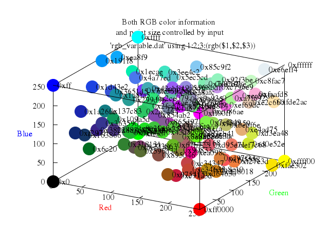
### 4
```ruby
# # Unfortunately, not all platforms allow us to read hexadecimal constants
# # from a data file. Warn the user if that is the case.
# #
# if (0 == int('0x01')) \
# set label 99 at screen .05, screen .15 "If you see only black dots,\nthis means your platform does not \nsupport reading hexadecimal constants\nfrom a data file. Get a newer libc."
#
# splot 'rgb_variable.dat' using 1:2:3:(5*rand(0)):4 with points pt 7 ps variable lc rgb variable \
# title "variable pointsize and rgb color read as hexidecimal"
Numo.gnuplot do
splot "'rgb_variable.dat'", using:'1:2:3:(5*rand(0)):4', with:"points", pt:7, ps:"variable", lc_rgb:"variable", title:"variable pointsize and rgb color read as hexidecimal"
end
```
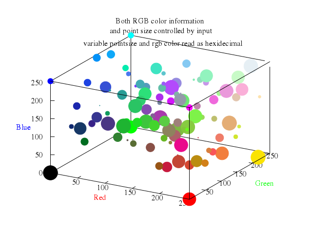
### 5
```ruby
# set label 99 ""
# #
# set border 0
# set xtics axis nomirror
# set ytics axis nomirror
# set ztics axis nomirror
# set xzeroaxis lt -1 lc rgb "red" lw 2
# set yzeroaxis lt -1 lc rgb "green" lw 2
# set zzeroaxis lt -1 lc rgb "blue" lw 2
# set xyplane at 0.0
#
# splot 'rgb_variable.dat' using 1:2:3:(5*rand(0)):(rgb($1,$2,$3)) with points pt 7 ps variable lc rgb variable \
# title "variable pointsize and rgb color computed from coords"
Numo.gnuplot do
set :label, 99, ""
set border:0
set :xtics, :axis, :nomirror
set :ytics, :axis, :nomirror
set :ztics, :axis, :nomirror
set :xzeroaxis, lt:-1, lc_rgb:"red", lw:2
set :yzeroaxis, lt:-1, lc_rgb:"green", lw:2
set :zzeroaxis, lt:-1, lc_rgb:"blue", lw:2
set :xyplane, at:0.0
splot "'rgb_variable.dat'", using:'1:2:3:(5*rand(0)):(rgb($1,$2,$3))', with:"points", pt:7, ps:"variable", lc_rgb:"variable", title:"variable pointsize and rgb color computed from coords"
end
```
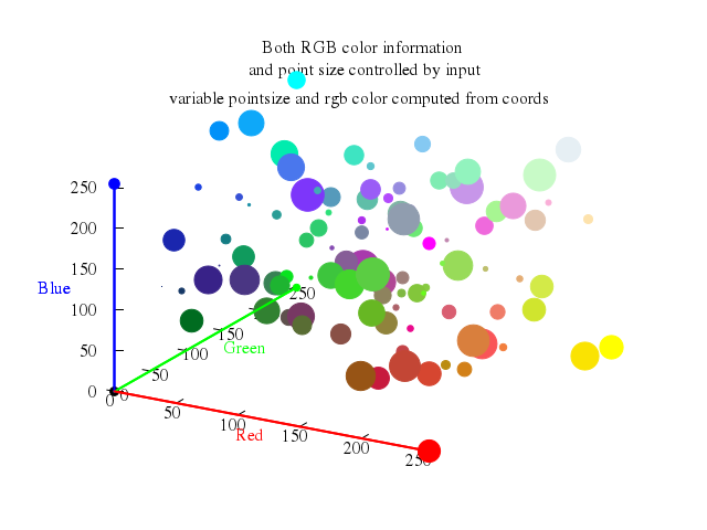
### 6
```ruby
# set title "Demo of hidden3d with points only (no surface)"
# set hidden3d
# replot
Numo.gnuplot do
set title:"Demo of hidden3d with points only (no surface)"
set :hidden3d
replot
end
```
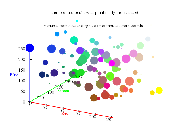
## pm3d colors
[Original Demo](http://gnuplot.sourceforge.net/demo_4.6/pm3dcolors.html)
### 1
```ruby
# # Test of color modes for pm3d palettes.
#
# #
# # Multiplot with some of the recommended rgbformulae palettes
# #
# set pm3d map
# set multiplot layout 3,3 \
# title "Palettes according to 'help palette rgbformulae'"
# g(x)=x
# set xrange [0:1]; set xtics 0.2 scale 1.5 nomirror; set mxtics 2
# # set palette maxcolors 128
# unset colorbox; unset key; set tics out; unset ytics
# set palette rgb 7,5,15; set title "traditional pm3d\n(black-blue-red-yellow)"; splot g(x)
# set palette rgb 3,11,6; set title "green-red-violet"; splot g(x)
# set palette rgb 23,28,3; set title "ocean (green-blue-white)\ntry also other permutations"; splot g(x)
# set palette rgb 21,22,23; set title "hot (black-red-yellow-white)"; splot g(x)
# set palette rgb 30,31,32; set title "color printable on gray\n(black-blue-violet-yellow-white)"; splot g(x)
# set palette rgb 33,13,10; set title "rainbow (blue-green-yellow-red)"; splot g(x)
# set palette rgb 34,35,36; set title "AFM hot (black-red-yellow-white)"; splot g(x)
# set palette model HSV
# set palette rgb 3,2,2; set title "HSV model\n(red-yellow-green-cyan-blue-magenta-red)"; splot g(x)
# set pal gray; set title "gray palette"; splot g(x)
# unset multiplot
Numo.gnuplot do
set :pm3d, :map
set :multiplot, layout:[3,3], title:"Palettes according to 'help palette rgbformulae'"
run "g(x)=x"
set xrange:0..1; set xtics:0.2, scale:1.5, nomirror:true; set mxtics:2
unset :colorbox; unset :key; set :tics, :out; unset :ytics
set :palette, rgb:[7,5,15]; set title:"traditional pm3d\n(black-blue-red-yellow)"; splot "g(x)"
set :palette, rgb:[3,11,6]; set title:"green-red-violet"; splot "g(x)"
set :palette, rgb:[23,28,3]; set title:"ocean (green-blue-white)\ntry also other permutations"; splot "g(x)"
set :palette, rgb:[21,22,23]; set title:"hot (black-red-yellow-white)"; splot "g(x)"
set :palette, rgb:[30,31,32]; set title:"color printable on gray\n(black-blue-violet-yellow-white)"; splot "g(x)"
set :palette, rgb:[33,13,10]; set title:"rainbow (blue-green-yellow-red)"; splot "g(x)"
set :palette, rgb:[34,35,36]; set title:"AFM hot (black-red-yellow-white)"; splot "g(x)"
set :palette, model:"HSV"
set :palette, rgb:[3,2,2]; set title:"HSV model\n(red-yellow-green-cyan-blue-magenta-red)"; splot "g(x)"
set :pal, "gray"; set title:"gray palette"; splot "g(x)"
unset :multiplot
end
```
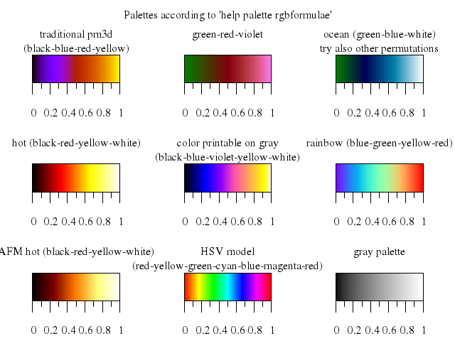
### 2
```ruby
# reset
#
# #
# # Gradient Palettes
# #
# set pm3d map
# set palette color
#
# f(x)=(x+10)/20
# set cbrange [f(-10):f(10)] # [0:1]
# set xrange [-10:10]
# set yrange [*:*]
# set xtics 2
# set cbtics 0.1
# set format cb "%3.1f"
# unset ztics
# unset ytics
# set samples 101
# set isosamples 2
# unset key
#
# set palette model RGB
#
# set palette defined
# set title "set palette defined"
# splot f(x)
Numo.gnuplot do
reset
set :pm3d, :map
set :palette, :color
run "f(x)=(x+10)/20"
set cbrange:"[f(-10):f(10)]" # [0:1]
set xrange:-10..10
set yrange:"[*:*]"
set xtics:2
set cbtics:0.1
set format_cb:"%3.1f"
unset :ztics
unset :ytics
set samples:101
set isosamples:2
unset :key
set :palette, model:"RGB"
set :palette, :defined
set title:"set palette defined"
splot "f(x)"
end
```
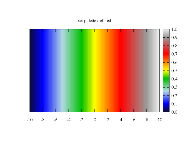
### 3
```ruby
# set palette defined (0 0 0 0, 1 0 0 1, 3 0 1 0, 4 1 0 0, 6 1 1 1)
# set title 'set palette defined (0 0 0 0, 1 0 0 1, 3 0 1 0, 4 1 0 0, 6 1 1 1)'
# splot f(x)
Numo.gnuplot do
set :palette, defined:'(0 0 0 0, 1 0 0 1, 3 0 1 0, 4 1 0 0, 6 1 1 1)'
set title:'set palette defined (0 0 0 0, 1 0 0 1, 3 0 1 0, 4 1 0 0, 6 1 1 1)'
splot "f(x)"
end
```
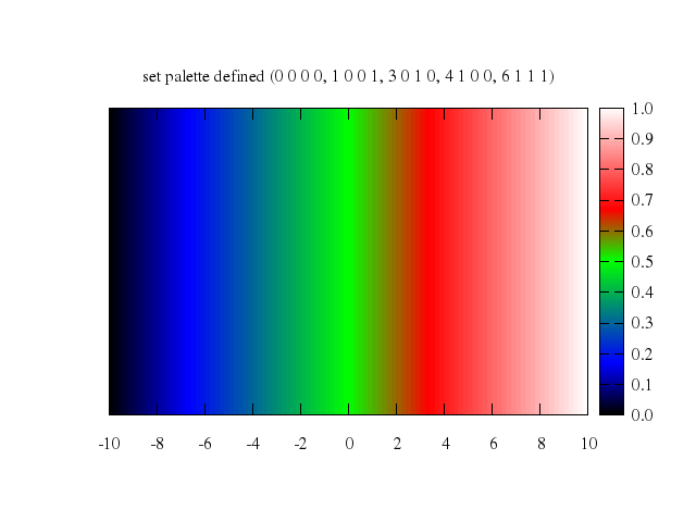
### 4
```ruby
# set palette defined ( 0 "green", 1 "blue", 2 "red", 3 "orange" )
# set title 'set palette defined ( 0 "green", 1 "blue", 2 "red", 3 "orange" )'
# splot f(x)
Numo.gnuplot do
set :palette, defined:'( 0 "green", 1 "blue", 2 "red", 3 "orange" )'
set title:'set palette defined ( 0 "green", 1 "blue", 2 "red", 3 "orange" )'
splot "f(x)"
end
```
### 5
```ruby
# set palette defined ( 20 "#101010", 30 "#ff0000", 40 "#00ff00", 50 "#e0e0e0" )
# set title 'set palette defined ( 20 "#101010", 30 "#ff0000", 40 "#00ff00", 50 "#e0e0e0" )'
# splot f(x)
Numo.gnuplot do
set :palette, defined:'( 20 "#101010", 30 "#ff0000", 40 "#00ff00", 50 "#e0e0e0" )'
set title:'set palette defined ( 20 "#101010", 30 "#ff0000", 40 "#00ff00", 50 "#e0e0e0" )'
splot "f(x)"
end
```
### 6
```ruby
# set palette defined ( 0 0 0 0, 1 1 1 1 )
# set title 'set palette defined ( 0 0 0 0, 1 1 1 1 )'
# splot f(x)
Numo.gnuplot do
set :palette, defined:'( 0 0 0 0, 1 1 1 1 )'
set title:'set palette defined ( 0 0 0 0, 1 1 1 1 )'
splot "f(x)"
end
```

### 7
```ruby
# set palette model HSV defined ( 0 0 1 1, 1 1 1 1 )
# set title 'set palette model HSV defined ( 0 0 1 1, 1 1 1 1 )'
# splot f(x)
Numo.gnuplot do
set :palette, model:"HSV", defined:'( 0 0 1 1, 1 1 1 1 )'
set title:'set palette model HSV defined ( 0 0 1 1, 1 1 1 1 )'
splot "f(x)"
end
```
### 8
```ruby
# set palette model RGB
# set palette model RGB defined (0 "green", 1 "dark-green", 1 "yellow", 2 "dark-yellow", 2 "red", 3 "dark-red" )
# set title "set palette model RGB defined\n(0 'green', 1 'dark-green', 1 'yellow', 2 'dark-yellow', 2 'red', 3 'dark-red' )"
# splot f(x)
Numo.gnuplot do
set :palette, model:"RGB"
set :palette, model:"RGB", defined:'(0 "green", 1 "dark-green", 1 "yellow", 2 "dark-yellow", 2 "red", 3 "dark-red" )'
set title:"set palette model RGB defined\n(0 'green', 1 'dark-green', 1 'yellow', 2 'dark-yellow', 2 'red', 3 'dark-red' )"
splot "f(x)"
end
```
### 9
```ruby
# set palette model RGB
#
# set title 'set palette file "-" (file with 3 columns)'
# set palette file "-"
# 0 0 0
# 0 0 1
# 0 1 0
# 1 0 0
# 1 1 1
# e
# splot f(x)
Numo.gnuplot do
set :palette, model:"RGB"
run < 7,5,15'
# splot f(x)
Numo.gnuplot do
set :palette, functions:'sqrt(gray),gray**3,sin(gray*2*pi)'
set title:'set palette functions sqrt(gray), gray**3, sin(gray*2*pi) <--> 7,5,15'
splot "f(x)"
end
```
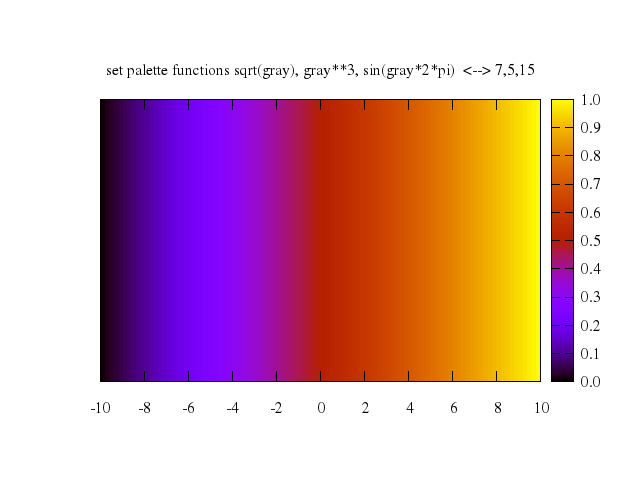
### 20
```ruby
# set palette rgbformulae 7,5,15
# set title 'set palette rgbformulae 7,5,15'
# splot f(x)
Numo.gnuplot do
set :palette, rgbformulae:[7,5,15]
set title:'set palette rgbformulae 7,5,15'
splot "f(x)"
end
```
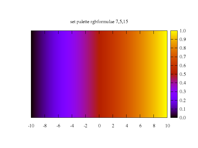
### 21
```ruby
# set palette model XYZ functions gray**0.35, gray**0.5, gray**0.8
# set title 'set palette model XYZ functions model XYZ gray**0.35, gray**0.5, gray**0.8'
# splot f(x)
Numo.gnuplot do
set :palette, model:"XYZ", functions:'gray**0.35,gray**0.5,gray**0.8'
set title:'set palette model XYZ functions model XYZ gray**0.35, gray**0.5, gray**0.8'
splot "f(x)"
end
```
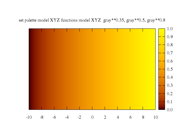
### 22
```ruby
# theta(x) = x<0 ? 0 : 1
# r(x) = 4*x*(1-theta(x-0.25))
# g(x) = 0.5*theta(x-0.25)*(1-theta(x-0.5))
# b(x) = x
# set palette model RGB functions r(gray),g(gray),b(gray)
# set title "set palette model RGB functions\n4*x*(1-theta(x-0.25)), 0.5*theta(x-0.25)*(1-theta(x-0.5)), x"
# splot f(x)
Numo.gnuplot do
run "theta(x) = x<0 ? 0 : 1"
run "r(x) = 4*x*(1-theta(x-0.25))"
run "g(x) = 0.5*theta(x-0.25)*(1-theta(x-0.5))"
run "b(x) = x"
set :palette, model:"RGB", functions:'r(gray),g(gray),b(gray)'
set title:"set palette model RGB functions\n4*x*(1-theta(x-0.25)), 0.5*theta(x-0.25)*(1-theta(x-0.5)), x"
splot "f(x)"
end
```
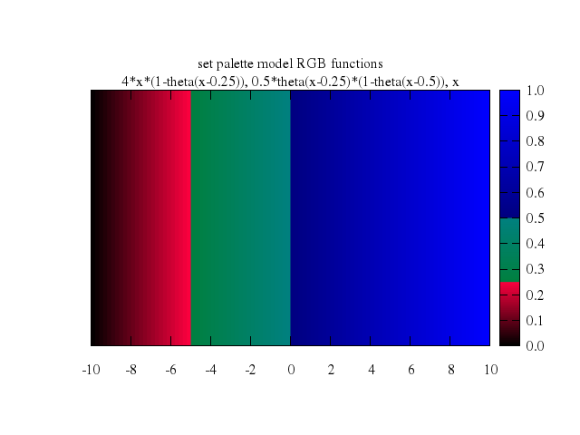
## pm3d gamma
[Original Demo](http://gnuplot.sourceforge.net/demo_4.6/pm3dgamma.html)
### 1
```ruby
# # Test of gamma correction for gray palettes
#
# set pm3d; set palette
# set palette gray
# set pm3d map
# set cbrange [-10:10]
# set xrange [-10:10]
# set yrange [*:*]
# unset ztics
# unset ytics
# set samples 101
# set isosamples 2
# set xtics 2
#
# set palette gamma 0.75
# set title "gamma = 0.75"
# splot x
Numo.gnuplot do
set :pm3d; set :palette
set :palette, "gray"
set :pm3d, :map
set cbrange:-10..10
set xrange:-10..10
set yrange:"[*:*]"
unset :ztics
unset :ytics
set samples:101
set isosamples:2
set xtics:2
set :palette, gamma:0.75
set title:"gamma = 0.75"
splot "x"
end
```

### 2
```ruby
# set palette gamma 1.0
# set title "gamma = 1.0"
# splot x
Numo.gnuplot do
set :palette, gamma:1.0
set title:"gamma = 1.0"
splot "x"
end
```

### 3
```ruby
# set palette gamma 1.25
# set title "gamma = 1.25"
# splot x
Numo.gnuplot do
set :palette, gamma:1.25
set title:"gamma = 1.25"
splot "x"
end
```

### 4
```ruby
# set palette gamma 1.5
# set title "gamma = 1.5"
# splot x
Numo.gnuplot do
set :palette, gamma:1.5
set title:"gamma = 1.5"
splot "x"
end
```

### 5
```ruby
# set palette gamma 1.75
# set title "gamma = 1.75"
# splot x
Numo.gnuplot do
set :palette, gamma:1.75
set title:"gamma = 1.75"
splot "x"
end
```
### 6
```ruby
# set palette gamma 2.0
# set title "gamma = 2.0"
# splot x
Numo.gnuplot do
set :palette, gamma:2.0
set title:"gamma = 2.0"
splot "x"
end
```
## control models
[Original Demo](http://gnuplot.sourceforge.net/demo_4.6/controls.html)
### 1
```ruby
# # warning: this demo is SLOW on PCs without math coprocessors!
# #
# # From _Automatic_Control_Systems_, fourth ed., figure 6-14
# # transient response of a second-order system to a unit step input function
# #
# damp(t) = exp(-s*wn*t)/sqrt(1.0-s*s)
# per(t) = sin(wn*sqrt(1.0-s**2)*t - atan(-sqrt(1.0-s**2)/s))
# c(t) = 1-damp(t)*per(t)
# #
# # wn is natural undamped frequency
# # s is damping factor
# #
# wn = 1.0
# set xrange [0:13]
# set samples 50
# set dummy t
# set key box
# #
# # plot c(t) for several different damping factors s
# #
# plot s=.1,c(t),s=.3,c(t),s=.5,c(t),s=.7,c(t),s=.9,c(t),s=1.0,c(t),s=1.5,c(t),s=2.0,c(t)
Numo.gnuplot do
run "damp(t) = exp(-s*wn*t)/sqrt(1.0-s*s)"
run "per(t) = sin(wn*sqrt(1.0-s**2)*t - atan(-sqrt(1.0-s**2)/s))"
run "c(t) = 1-damp(t)*per(t)"
run "wn = 1.0"
set xrange:0..13
set samples:50
set dummy:"t"
set :key, :box
plot "s=.1",
"c(t)",
"s=.3",
"c(t)",
"s=.5",
"c(t)",
"s=.7",
"c(t)",
"s=.9",
"c(t)",
"s=1.0",
"c(t)",
"s=1.5",
"c(t)",
"s=2.0",
"c(t)"
end
```
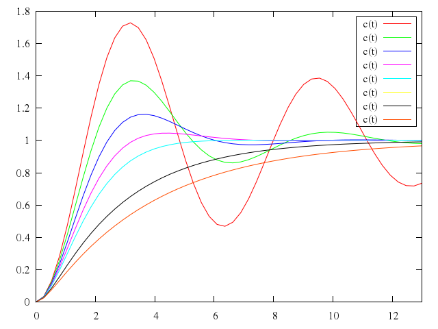
## discrete contours
[Original Demo](http://gnuplot.sourceforge.net/demo_4.6/discrete.html)
### 1
```ruby
# set contour
# set title "Demo of specifying discrete contour levels - default contours"
# splot x*y
Numo.gnuplot do
set :contour
set title:"Demo of specifying discrete contour levels - default contours"
splot "x*y"
end
```
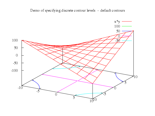
### 2
```ruby
# #set discrete levels
# set cntrparam levels discrete 0, 15, 75
# set title "3 discrete contours at 0 15 & 75"
# replot
Numo.gnuplot do
set :cntrparam, :levels, discrete:[0,15,75]
set title:"3 discrete contours at 0 15 & 75"
replot
end
```
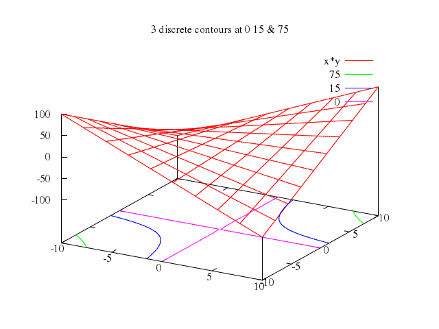
### 3
```ruby
# #set incremental levels
# set cntrp level incr -20, 5, 9
# set title "9 incremental contours starting at -20, stepping by 5"
# replot
Numo.gnuplot do
set :cntrp, :level, incr:[-20,5,9]
set title:"9 incremental contours starting at -20, stepping by 5"
replot
end
```
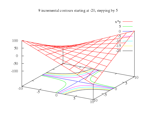
## financial data
[Original Demo](http://gnuplot.sourceforge.net/demo_4.6/finance.html)
### 1
```ruby
# # 10 May 2005
# #
# # Though gnuplot is primarily a scientific plotting program, it can do a great
# # job of plotting finance charts as well. The primary challenge is the irregular
# # nature of financial time series. Stocks don't trade every day, so when you set
# # the x-axis to time gaps appear for non-trading days. Investors and traders
# # generally prefer that these gaps be omitted. Another challenge is that finance
# # charts are best presented in semi-log form (log y-axis, linear x-axis),
# # but gnuplot wants to span decades in its log scaling, something that stocks
# # rarely do. These and other challenges are met in finance.dem, a short
# # demonstration script that proves that gnuplot can really shine in this area.
# #
# # gnuplot plays a central role in our work. Almost all the graphs in "Bollinger
# # on Bollinger Bands" were plotted by gnuplot, many gnuplot visuals have
# # appeared on CNBC, our in-house analytics use gnuplot for visual display and
# # The Capital Growth Letter relies heavily on gnuplot for its charts.
# #
# # Finally, gnuplot is yet another successful demonstration of a powerful idea,
# # open source programming. Thanks to all who made gnuplot possible from the
# # earliest days to the present and to all those who will contribute in the
# # future. (Special thanks to Hans-Bernhard Broeker whose patience helped me to
# # climb the grade and to Ethan Merritt whose recent contributions have been
# # invaluable to our work.)
# #
# # John Bollinger
# # www.BollingerBands.com
#
# # a demonstration of gnuplot finance plot styles
# # by John Bollinger, CFA, CMT
# # www.BollingerBands.com
# # [email protected]
#
# # data and indicators in finance.dat
# # data file layout:
# # date, open, high, low, close, volume,
# # 50-day moving average volume, Intraday Intensity,
# # 20-day moving average close,
# # upper Bollinger Band, lower Bollinger Band
#
# # last update: 8 May 2005
#
# reset
# # set label 1 "Demo of plotting financial data" at screen 0.5, screen 0.95 center
# set title "Demo of plotting financial data"
# set yrange [75:105]
# set ytics (105, 100, 95, 90, 85, 80)
# set xrange [50:253]
# set lmargin 9
# set rmargin 2
# plot 'finance.dat' using 0:5 notitle with lines
Numo.gnuplot do
reset
set title:"Demo of plotting financial data"
set yrange:75..105
set ytics:'(105, 100, 95, 90, 85, 80)'
set xrange:50..253
set lmargin:9
set rmargin:2
plot "'finance.dat'", using:[0,5], notitle:true, with:"lines"
end
```
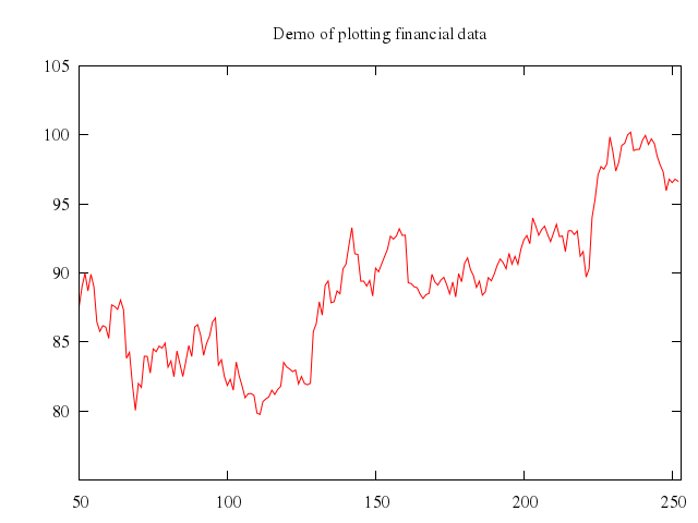
### 2
```ruby
# reset
# set title "Turn on grid"
# set yrange [75:105]
# set ytics (105, 100, 95, 90, 85, 80)
# set xrange [50:253]
# set lmargin 9
# set rmargin 2
# set grid
# plot 'finance.dat' using 0:5 notitle with lines
Numo.gnuplot do
reset
set title:"Turn on grid"
set yrange:75..105
set ytics:'(105, 100, 95, 90, 85, 80)'
set xrange:50..253
set lmargin:9
set rmargin:2
set :grid
plot "'finance.dat'", using:[0,5], notitle:true, with:"lines"
end
```
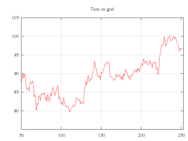
### 3
```ruby
# reset
# set title "Semi-log scaling"
# set yrange [75:105]
# set ytics (105, 100, 95, 90, 85, 80)
# set xrange [50:253]
# set lmargin 9
# set rmargin 2
# set grid
# set logscale y
# plot 'finance.dat' using 0:5 notitle with lines
Numo.gnuplot do
reset
set title:"Semi-log scaling"
set yrange:75..105
set ytics:'(105, 100, 95, 90, 85, 80)'
set xrange:50..253
set lmargin:9
set rmargin:2
set :grid
set logscale:"y"
plot "'finance.dat'", using:[0,5], notitle:true, with:"lines"
end
```
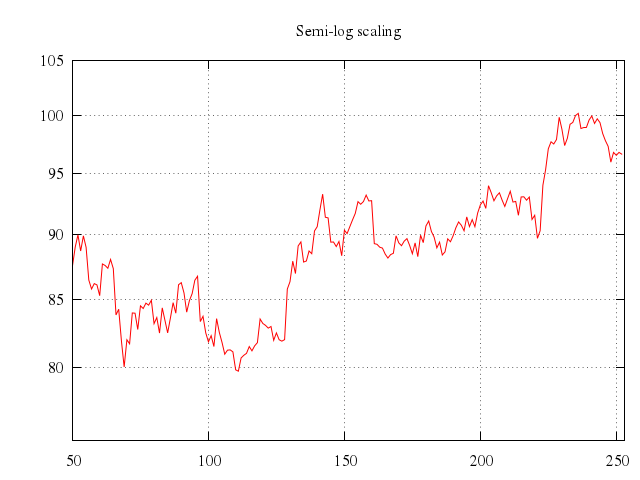
### 4
```ruby
# reset
# set title "Finance bars"
# set yrange [75:105]
# set ytics (105, 100, 95, 90, 85, 80)
# set xrange [50:253]
# set lmargin 9
# set rmargin 2
# set grid
# set logscale y
# plot 'finance.dat' using 0:2:3:4:5 notitle with financebars lt 8
Numo.gnuplot do
reset
set title:"Finance bars"
set yrange:75..105
set ytics:'(105, 100, 95, 90, 85, 80)'
set xrange:50..253
set lmargin:9
set rmargin:2
set :grid
set logscale:"y"
plot "'finance.dat'", using:[0,2,3,4,5], notitle:true, with:"financebars", lt:8
end
```
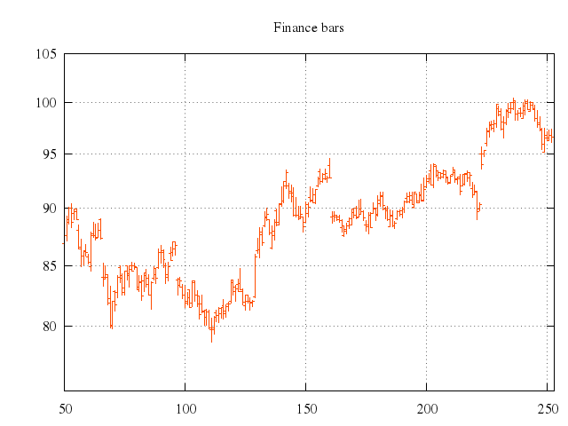
### 5
```ruby
# reset
# set title "Bollinger Bands"
# set yrange [75:105]
# set ytics (105, 100, 95, 90, 85, 80)
# set xrange [50:253]
# set lmargin 9
# set rmargin 2
# set grid
# set logscale y
# plot 'finance.dat' using 0:2:3:4:5 notitle with financebars lt 8, \
# 'finance.dat' using 0:9 notitle with lines lt 3, \
# 'finance.dat' using 0:10 notitle with lines lt 1, \
# 'finance.dat' using 0:11 notitle with lines lt 2
Numo.gnuplot do
reset
set title:"Bollinger Bands"
set yrange:75..105
set ytics:'(105, 100, 95, 90, 85, 80)'
set xrange:50..253
set lmargin:9
set rmargin:2
set :grid
set logscale:"y"
plot ["'finance.dat'", using:[0,2,3,4,5], notitle:true, with:"financebars", lt:8],
["'finance.dat'", using:[0,9], notitle:true, with:"lines", lt:3],
["'finance.dat'", using:[0,10], notitle:true, with:"lines", lt:1],
["'finance.dat'", using:[0,11], notitle:true, with:"lines", lt:2]
end
```
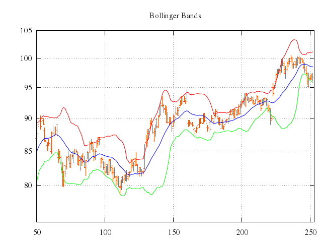
### 6
```ruby
# reset
# set title "Overlay an indicator on a separate scale"
# set yrange [75:105]
# set ytics (105, 100, 95, 90, 85, 80)
# set xrange [50:253]
# set lmargin 9
# set rmargin 2
# set grid
# set logscale y
# plot 'finance.dat' using 0:2:3:4:5 notitle with financebars lt 8, \
# 'finance.dat' using 0:9 notitle with lines lt 3, \
# 'finance.dat' using 0:10 notitle with lines lt 1, \
# 'finance.dat' using 0:11 notitle with lines lt 2, \
# 'finance.dat' using 0:8 axes x1y2 notitle with lines lt 4
Numo.gnuplot do
reset
set title:"Overlay an indicator on a separate scale"
set yrange:75..105
set ytics:'(105, 100, 95, 90, 85, 80)'
set xrange:50..253
set lmargin:9
set rmargin:2
set :grid
set logscale:"y"
plot ["'finance.dat'", using:[0,2,3,4,5], notitle:true, with:"financebars", lt:8],
["'finance.dat'", using:[0,9], notitle:true, with:"lines", lt:3],
["'finance.dat'", using:[0,10], notitle:true, with:"lines", lt:1],
["'finance.dat'", using:[0,11], notitle:true, with:"lines", lt:2],
["'finance.dat'", using:[0,8], axes:"x1y2", notitle:true, with:"lines", lt:4]
end
```
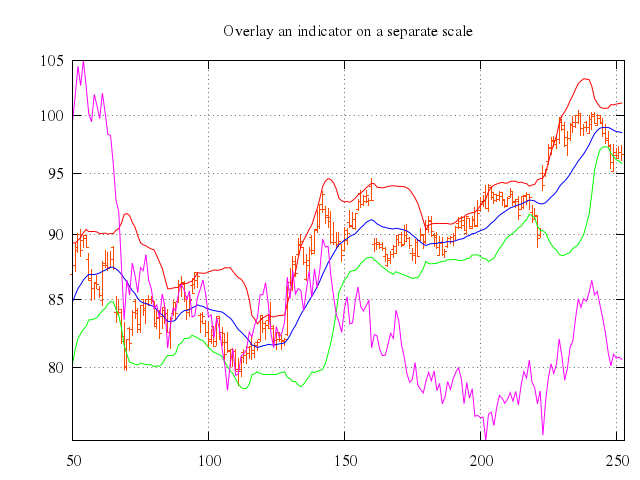
### 7
```ruby
# reset
# set title "Add some boiler plate"
# set label "Courtesy of Bollinger Capital" at graph 0.01, 0.07
# set label " www.BollingerBands.com" at graph 0.01, 0.03
# set yrange [75:105]
# set ytics (105, 100, 95, 90, 85, 80)
# set xrange [50:253]
# set lmargin 9
# set rmargin 2
# set grid
# set logscale y
# plot 'finance.dat' using 0:2:3:4:5 notitle with financebars lt 8, \
# 'finance.dat' using 0:9 notitle with lines lt 3, \
# 'finance.dat' using 0:10 notitle with lines lt 1, \
# 'finance.dat' using 0:11 notitle with lines lt 2, \
# 'finance.dat' using 0:8 axes x1y2 notitle with lines lt 4
Numo.gnuplot do
reset
set title:"Add some boiler plate"
set label:"Courtesy of Bollinger Capital", at_graph:[0.01,0.07]
set label:" www.BollingerBands.com", at_graph:[0.01,0.03]
set yrange:75..105
set ytics:'(105, 100, 95, 90, 85, 80)'
set xrange:50..253
set lmargin:9
set rmargin:2
set :grid
set logscale:"y"
plot ["'finance.dat'", using:[0,2,3,4,5], notitle:true, with:"financebars", lt:8],
["'finance.dat'", using:[0,9], notitle:true, with:"lines", lt:3],
["'finance.dat'", using:[0,10], notitle:true, with:"lines", lt:1],
["'finance.dat'", using:[0,11], notitle:true, with:"lines", lt:2],
["'finance.dat'", using:[0,8], axes:"x1y2", notitle:true, with:"lines", lt:4]
end
```
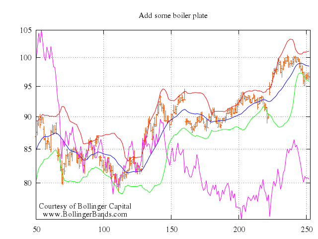
### 8
```ruby
# reset
# set label "Courtesy of Bollinger Capital" at graph 0.01, 0.07
# set label " www.BollingerBands.com" at graph 0.01, 0.03
# set logscale y
# set yrange [75:105]
# set ytics (105, 100, 95, 90, 85, 80)
# set xrange [50:253]
# set grid
# set lmargin 9
# set rmargin 2
# set format x ""
# set xtics (66, 87, 109, 130, 151, 174, 193, 215, 235)
# set multiplot
# set size 1, 0.7
# set origin 0, 0.3
# set bmargin 0
# set title "Add volume in a separate clip"
# plot 'finance.dat' using 0:2:3:4:5 notitle with financebars lt 8, \
# 'finance.dat' using 0:9 notitle with lines lt 3, \
# 'finance.dat' using 0:10 notitle with lines lt 1, \
# 'finance.dat' using 0:11 notitle with lines lt 2, \
# 'finance.dat' using 0:8 axes x1y2 notitle with lines lt 4
# unset label 1
# unset label 2
# unset title
# set bmargin
# set format x
# set size 1.0, 0.3
# set origin 0.0, 0.0
# set tmargin 0
# unset logscale y
# set autoscale y
# set format y "%1.0f"
# set ytics 500
# plot 'finance.dat' using 0:($6/10000) notitle with impulses lt 3
# unset multiplot
Numo.gnuplot do
reset
set label:"Courtesy of Bollinger Capital", at_graph:[0.01,0.07]
set label:" www.BollingerBands.com", at_graph:[0.01,0.03]
set logscale:"y"
set yrange:75..105
set ytics:'(105, 100, 95, 90, 85, 80)'
set xrange:50..253
set :grid
set lmargin:9
set rmargin:2
set format_x:""
set xtics:'(66, 87, 109, 130, 151, 174, 193, 215, 235)'
set :multiplot
set size:[1,0.7]
set origin:[0,0.3]
set bmargin:0
set title:"Add volume in a separate clip"
plot ["'finance.dat'", using:[0,2,3,4,5], notitle:true, with:"financebars", lt:8],
["'finance.dat'", using:[0,9], notitle:true, with:"lines", lt:3],
["'finance.dat'", using:[0,10], notitle:true, with:"lines", lt:1],
["'finance.dat'", using:[0,11], notitle:true, with:"lines", lt:2],
["'finance.dat'", using:[0,8], axes:"x1y2", notitle:true, with:"lines", lt:4]
unset label:1
unset label:2
unset :title
set :bmargin
set format:"x"
set size:[1.0,0.3]
set origin:[0.0,0.0]
set tmargin:0
unset logscale:"y"
set autoscale:"y"
set format_y:"%1.0f"
set ytics:500
plot "'finance.dat'", using:'0:($6/10000)', notitle:true, with:"impulses", lt:3
unset :multiplot
end
```
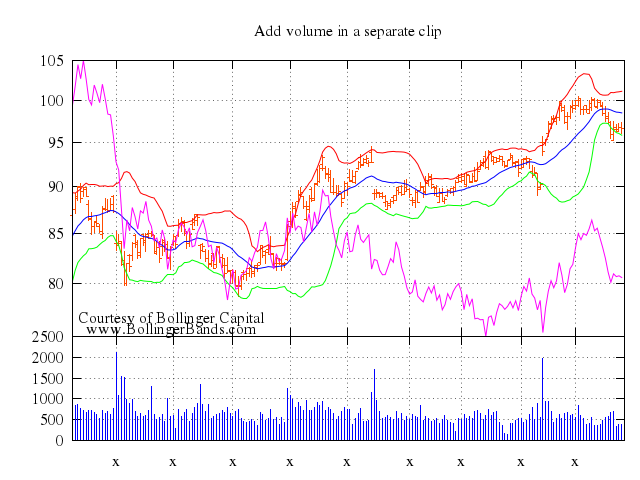
### 9
```ruby
# reset
# set label "Courtesy of Bollinger Capital" at graph 0.01, 0.07
# set label " www.BollingerBands.com" at graph 0.01, 0.03
# set logscale y
# set yrange [75:105]
# set ytics (105, 100, 95, 90, 85, 80)
# set xrange [50:253]
# set grid
# set lmargin 9
# set rmargin 2
# set format x ""
# set xtics (66, 87, 109, 130, 151, 174, 193, 215, 235)
# set multiplot
# set title "Add average volume"
# set size 1, 0.7
# set origin 0, 0.3
# set bmargin 0
# plot 'finance.dat' using 0:2:3:4:5 notitle with financebars lt 8, \
# 'finance.dat' using 0:9 notitle with lines lt 3, \
# 'finance.dat' using 0:10 notitle with lines lt 1, \
# 'finance.dat' using 0:11 notitle with lines lt 2, \
# 'finance.dat' using 0:8 axes x1y2 notitle with lines lt 4
# unset label 1
# unset label 2
# unset title
# set bmargin
# set format x
# set size 1.0, 0.3
# set origin 0.0, 0.0
# set tmargin 0
# unset logscale y
# set autoscale y
# set format y "%1.0f"
# set ytics 500
# plot 'finance.dat' using 0:($6/10000) notitle with impulses lt 3, \
# 'finance.dat' using 0:($7/10000) notitle with lines lt 1
# unset multiplot
Numo.gnuplot do
reset
set label:"Courtesy of Bollinger Capital", at_graph:[0.01,0.07]
set label:" www.BollingerBands.com", at_graph:[0.01,0.03]
set logscale:"y"
set yrange:75..105
set ytics:'(105, 100, 95, 90, 85, 80)'
set xrange:50..253
set :grid
set lmargin:9
set rmargin:2
set format_x:""
set xtics:'(66, 87, 109, 130, 151, 174, 193, 215, 235)'
set :multiplot
set title:"Add average volume"
set size:[1,0.7]
set origin:[0,0.3]
set bmargin:0
plot ["'finance.dat'", using:[0,2,3,4,5], notitle:true, with:"financebars", lt:8],
["'finance.dat'", using:[0,9], notitle:true, with:"lines", lt:3],
["'finance.dat'", using:[0,10], notitle:true, with:"lines", lt:1],
["'finance.dat'", using:[0,11], notitle:true, with:"lines", lt:2],
["'finance.dat'", using:[0,8], axes:"x1y2", notitle:true, with:"lines", lt:4]
unset label:1
unset label:2
unset :title
set :bmargin
set format:"x"
set size:[1.0,0.3]
set origin:[0.0,0.0]
set tmargin:0
unset logscale:"y"
set autoscale:"y"
set format_y:"%1.0f"
set ytics:500
plot ["'finance.dat'", using:'0:($6/10000)', notitle:true, with:"impulses", lt:3],
["'finance.dat'", using:'0:($7/10000)', notitle:true, with:"lines", lt:1]
unset :multiplot
end
```
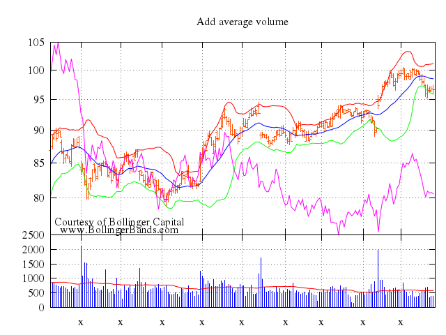
### 10
```ruby
# reset
# set label "Courtesy of Bollinger Capital" at graph 0.01, 0.07
# set label " www.BollingerBands.com" at graph 0.01, 0.03
# set logscale y
# set yrange [75:105]
# set ytics (105, 100, 95, 90, 85, 80)
# set xrange [50:253]
# set grid
# set lmargin 9
# set rmargin 2
# set format x ""
# set xtics (66, 87, 109, 130, 151, 174, 193, 215, 235)
# set multiplot
# set title "Add date labels to the x axis"
# set size 1, 0.7
# set origin 0, 0.3
# set bmargin 0
# plot 'finance.dat' using 0:2:3:4:5 notitle with financebars lt 8, \
# 'finance.dat' using 0:9 notitle with lines lt 3, \
# 'finance.dat' using 0:10 notitle with lines lt 1, \
# 'finance.dat' using 0:11 notitle with lines lt 2, \
# 'finance.dat' using 0:8 axes x1y2 notitle with lines lt 4
# unset label 1
# unset label 2
# unset title
# set bmargin
# set format x
# set size 1.0, 0.3
# set origin 0.0, 0.0
# set tmargin 0
# unset logscale y
# set autoscale y
# set format y "%1.0f"
# set ytics 500
# set xtics ("6/03" 66, "7/03" 87, "8/03" 109, "9/03" 130, "10/03" 151, "11/03" 174, "12/03" 193, "1/04" 215, "2/04" 235)
# plot 'finance.dat' using 0:($6/10000) notitle with impulses lt 3, \
# 'finance.dat' using 0:($7/10000) notitle with lines lt 1
# unset multiplot
Numo.gnuplot do
reset
set label:"Courtesy of Bollinger Capital", at_graph:[0.01,0.07]
set label:" www.BollingerBands.com", at_graph:[0.01,0.03]
set logscale:"y"
set yrange:75..105
set ytics:'(105, 100, 95, 90, 85, 80)'
set xrange:50..253
set :grid
set lmargin:9
set rmargin:2
set format_x:""
set xtics:'(66, 87, 109, 130, 151, 174, 193, 215, 235)'
set :multiplot
set title:"Add date labels to the x axis"
set size:[1,0.7]
set origin:[0,0.3]
set bmargin:0
plot ["'finance.dat'", using:[0,2,3,4,5], notitle:true, with:"financebars", lt:8],
["'finance.dat'", using:[0,9], notitle:true, with:"lines", lt:3],
["'finance.dat'", using:[0,10], notitle:true, with:"lines", lt:1],
["'finance.dat'", using:[0,11], notitle:true, with:"lines", lt:2],
["'finance.dat'", using:[0,8], axes:"x1y2", notitle:true, with:"lines", lt:4]
unset label:1
unset label:2
unset :title
set :bmargin
set format:"x"
set size:[1.0,0.3]
set origin:[0.0,0.0]
set tmargin:0
unset logscale:"y"
set autoscale:"y"
set format_y:"%1.0f"
set ytics:500
set xtics:'("6/03" 66, "7/03" 87, "8/03" 109, "9/03" 130, "10/03" 151, "11/03" 174, "12/03" 193, "1/04" 215, "2/04" 235)'
plot ["'finance.dat'", using:'0:($6/10000)', notitle:true, with:"impulses", lt:3],
["'finance.dat'", using:'0:($7/10000)', notitle:true, with:"lines", lt:1]
unset :multiplot
end
```
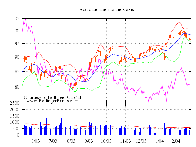
### 11
```ruby
# reset
# set label "Courtesy of Bollinger Capital" at graph 0.01, 0.07
# set label " www.BollingerBands.com" at graph 0.01, 0.03
# set logscale y
# set yrange [75:105]
# set ytics (105, 100, 95, 90, 85, 80)
# set xrange [50:253]
# set grid
# set lmargin 9
# set rmargin 2
# set format x ""
# set xtics (66, 87, 109, 130, 151, 174, 193, 215, 235)
# set multiplot
# set title "Add labels for each clip"
# set size 1, 0.7
# set origin 0, 0.3
# set bmargin 0
# set ylabel "price" offset 1
# plot 'finance.dat' using 0:2:3:4:5 notitle with financebars lt 8, \
# 'finance.dat' using 0:9 notitle with lines lt 3, \
# 'finance.dat' using 0:10 notitle with lines lt 1, \
# 'finance.dat' using 0:11 notitle with lines lt 2, \
# 'finance.dat' using 0:8 axes x1y2 notitle with lines lt 4
# unset label 1
# unset label 2
# unset title
# set bmargin
# set format x
# set size 1.0, 0.3
# set origin 0.0, 0.0
# set tmargin 0
# unset logscale y
# set autoscale y
# set format y "%1.0f"
# set ytics 500
# set xtics ("6/03" 66, "7/03" 87, "8/03" 109, "9/03" 130, "10/03" 151, "11/03" 174, "12/03" 193, "1/04" 215, "2/04" 235)
# set ylabel "volume (0000)" offset 1
# plot 'finance.dat' using 0:($6/10000) notitle with impulses lt 3, \
# 'finance.dat' using 0:($7/10000) notitle with lines lt 1
# unset multiplot
Numo.gnuplot do
reset
set label:"Courtesy of Bollinger Capital", at_graph:[0.01,0.07]
set label:" www.BollingerBands.com", at_graph:[0.01,0.03]
set logscale:"y"
set yrange:75..105
set ytics:'(105, 100, 95, 90, 85, 80)'
set xrange:50..253
set :grid
set lmargin:9
set rmargin:2
set format_x:""
set xtics:'(66, 87, 109, 130, 151, 174, 193, 215, 235)'
set :multiplot
set title:"Add labels for each clip"
set size:[1,0.7]
set origin:[0,0.3]
set bmargin:0
set ylabel:"price", offset:1
plot ["'finance.dat'", using:[0,2,3,4,5], notitle:true, with:"financebars", lt:8],
["'finance.dat'", using:[0,9], notitle:true, with:"lines", lt:3],
["'finance.dat'", using:[0,10], notitle:true, with:"lines", lt:1],
["'finance.dat'", using:[0,11], notitle:true, with:"lines", lt:2],
["'finance.dat'", using:[0,8], axes:"x1y2", notitle:true, with:"lines", lt:4]
unset label:1
unset label:2
unset :title
set :bmargin
set format:"x"
set size:[1.0,0.3]
set origin:[0.0,0.0]
set tmargin:0
unset logscale:"y"
set autoscale:"y"
set format_y:"%1.0f"
set ytics:500
set xtics:'("6/03" 66, "7/03" 87, "8/03" 109, "9/03" 130, "10/03" 151, "11/03" 174, "12/03" 193, "1/04" 215, "2/04" 235)'
set ylabel:"volume (0000)", offset:1
plot ["'finance.dat'", using:'0:($6/10000)', notitle:true, with:"impulses", lt:3],
["'finance.dat'", using:'0:($7/10000)', notitle:true, with:"lines", lt:1]
unset :multiplot
end
```
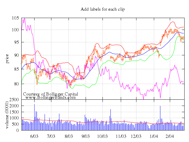
### 12
```ruby
# reset
# set label 1 "Acme Widgets" at graph 0.5, graph 0.9 center front
# set label 2 "Courtesy of Bollinger Capital" at graph 0.01, 0.07
# set label 3 " www.BollingerBands.com" at graph 0.01, 0.03
# set logscale y
# set yrange [75:105]
# set ytics (105, 100, 95, 90, 85, 80)
# set xrange [50:253]
# set grid
# set lmargin 9
# set rmargin 2
# set format x ""
# set xtics (66, 87, 109, 130, 151, 174, 193, 215, 235)
# set multiplot
# set title "Add a title"
# set size 1, 0.7
# set origin 0, 0.3
# set bmargin 0
# set ylabel "price" offset 1
# plot 'finance.dat' using 0:2:3:4:5 notitle with financebars lt 8, \
# 'finance.dat' using 0:9 notitle with lines lt 3, \
# 'finance.dat' using 0:10 notitle with lines lt 1, \
# 'finance.dat' using 0:11 notitle with lines lt 2, \
# 'finance.dat' using 0:8 axes x1y2 notitle with lines lt 4
# unset label 1
# unset label 2
# unset label 3
# unset title
# set bmargin
# set format x
# set size 1.0, 0.3
# set origin 0.0, 0.0
# set tmargin 0
# unset logscale y
# set autoscale y
# set format y "%1.0f"
# set ytics 500
# set xtics ("6/03" 66, "7/03" 87, "8/03" 109, "9/03" 130, "10/03" 151, "11/03" 174, "12/03" 193, "1/04" 215, "2/04" 235)
# set ylabel "volume (0000)" offset 1
# plot 'finance.dat' using 0:($6/10000) notitle with impulses lt 3, \
# 'finance.dat' using 0:($7/10000) notitle with lines lt 1
# unset multiplot
Numo.gnuplot do
reset
set :label, 1, "Acme Widgets", at:"graph 0.5, graph 0.9", center:true, front:true
set :label, 2, "Courtesy of Bollinger Capital", at_graph:[0.01,0.07]
set :label, 3, " www.BollingerBands.com", at_graph:[0.01,0.03]
set logscale:"y"
set yrange:75..105
set ytics:'(105, 100, 95, 90, 85, 80)'
set xrange:50..253
set :grid
set lmargin:9
set rmargin:2
set format_x:""
set xtics:'(66, 87, 109, 130, 151, 174, 193, 215, 235)'
set :multiplot
set title:"Add a title"
set size:[1,0.7]
set origin:[0,0.3]
set bmargin:0
set ylabel:"price", offset:1
plot ["'finance.dat'", using:[0,2,3,4,5], notitle:true, with:"financebars", lt:8],
["'finance.dat'", using:[0,9], notitle:true, with:"lines", lt:3],
["'finance.dat'", using:[0,10], notitle:true, with:"lines", lt:1],
["'finance.dat'", using:[0,11], notitle:true, with:"lines", lt:2],
["'finance.dat'", using:[0,8], axes:"x1y2", notitle:true, with:"lines", lt:4]
unset label:1
unset label:2
unset label:3
unset :title
set :bmargin
set format:"x"
set size:[1.0,0.3]
set origin:[0.0,0.0]
set tmargin:0
unset logscale:"y"
set autoscale:"y"
set format_y:"%1.0f"
set ytics:500
set xtics:'("6/03" 66, "7/03" 87, "8/03" 109, "9/03" 130, "10/03" 151, "11/03" 174, "12/03" 193, "1/04" 215, "2/04" 235)'
set ylabel:"volume (0000)", offset:1
plot ["'finance.dat'", using:'0:($6/10000)', notitle:true, with:"impulses", lt:3],
["'finance.dat'", using:'0:($7/10000)', notitle:true, with:"lines", lt:1]
unset :multiplot
end
```
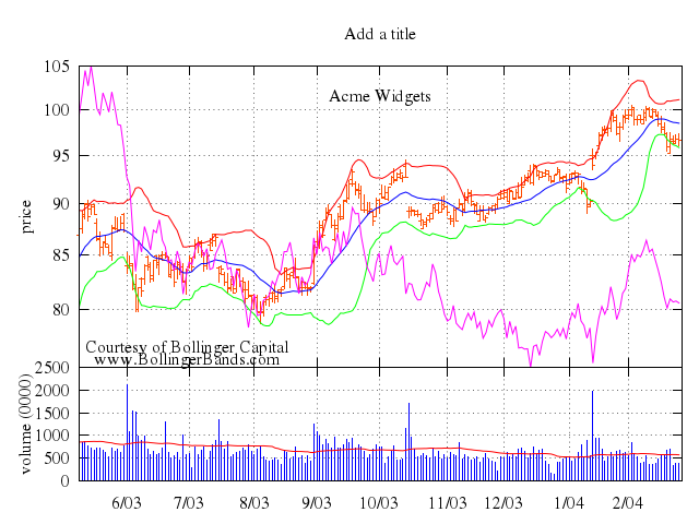
### 13
```ruby
# reset
# set label 1 "Acme Widgets" at graph 0.5, graph 0.9 center front
# set label 2 "Courtesy of Bollinger Capital" at graph 0.01, 0.07
# set label 3 " www.BollingerBands.com" at graph 0.01, 0.03
# set logscale y
# set yrange [75:105]
# set ytics (105, 100, 95, 90, 85, 80)
# set xrange [50:253]
# set grid
# set lmargin 9
# set rmargin 2
# set format x ""
# set xtics (66, 87, 109, 130, 151, 174, 193, 215, 235)
# set multiplot
# set title "Change to candlesticks"
# set size 1, 0.7
# set origin 0, 0.3
# set bmargin 0
# set ylabel "price" offset 1
# plot 'finance.dat' using 0:2:3:4:5 notitle with candlesticks lt 8, \
# 'finance.dat' using 0:9 notitle with lines lt 3, \
# 'finance.dat' using 0:10 notitle with lines lt 1, \
# 'finance.dat' using 0:11 notitle with lines lt 2, \
# 'finance.dat' using 0:8 axes x1y2 notitle with lines lt 4
# unset label 1
# unset label 2
# unset label 3
# unset title
# set bmargin
# set format x
# set size 1.0, 0.3
# set origin 0.0, 0.0
# set tmargin 0
# unset logscale y
# set autoscale y
# set format y "%1.0f"
# set ytics 500
# set xtics ("6/03" 66, "7/03" 87, "8/03" 109, "9/03" 130, "10/03" 151, "11/03" 174, "12/03" 193, "1/04" 215, "2/04" 235)
# set ylabel "volume (0000)" offset 1
# plot 'finance.dat' using 0:($6/10000) notitle with impulses lt 3, \
# 'finance.dat' using 0:($7/10000) notitle with lines lt 1
# unset multiplot
Numo.gnuplot do
reset
set :label, 1, "Acme Widgets", at:"graph 0.5, graph 0.9", center:true, front:true
set :label, 2, "Courtesy of Bollinger Capital", at_graph:[0.01,0.07]
set :label, 3, " www.BollingerBands.com", at_graph:[0.01,0.03]
set logscale:"y"
set yrange:75..105
set ytics:'(105, 100, 95, 90, 85, 80)'
set xrange:50..253
set :grid
set lmargin:9
set rmargin:2
set format_x:""
set xtics:'(66, 87, 109, 130, 151, 174, 193, 215, 235)'
set :multiplot
set title:"Change to candlesticks"
set size:[1,0.7]
set origin:[0,0.3]
set bmargin:0
set ylabel:"price", offset:1
plot ["'finance.dat'", using:[0,2,3,4,5], notitle:true, with:"candlesticks", lt:8],
["'finance.dat'", using:[0,9], notitle:true, with:"lines", lt:3],
["'finance.dat'", using:[0,10], notitle:true, with:"lines", lt:1],
["'finance.dat'", using:[0,11], notitle:true, with:"lines", lt:2],
["'finance.dat'", using:[0,8], axes:"x1y2", notitle:true, with:"lines", lt:4]
unset label:1
unset label:2
unset label:3
unset :title
set :bmargin
set format:"x"
set size:[1.0,0.3]
set origin:[0.0,0.0]
set tmargin:0
unset logscale:"y"
set autoscale:"y"
set format_y:"%1.0f"
set ytics:500
set xtics:'("6/03" 66, "7/03" 87, "8/03" 109, "9/03" 130, "10/03" 151, "11/03" 174, "12/03" 193, "1/04" 215, "2/04" 235)'
set ylabel:"volume (0000)", offset:1
plot ["'finance.dat'", using:'0:($6/10000)', notitle:true, with:"impulses", lt:3],
["'finance.dat'", using:'0:($7/10000)', notitle:true, with:"lines", lt:1]
unset :multiplot
end
```
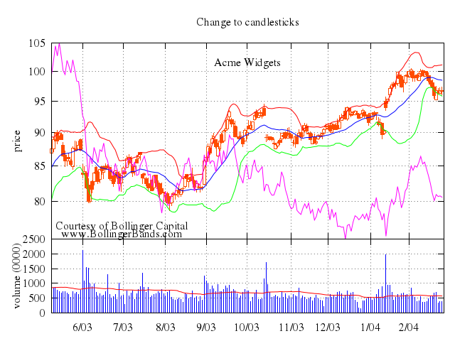
### 14
```ruby
# reset
# set label 1 "Acme Widgets" at graph 0.5, graph 0.9 center front
# set label 2 "Courtesy of Bollinger Capital" at graph 0.01, 0.07
# set label 3 " www.BollingerBands.com" at graph 0.01, 0.03
# set logscale y
# set yrange [75:105]
# set ytics (105, 100, 95, 90, 85, 80)
# set xrange [50:253]
# set grid
# set lmargin 9
# set rmargin 2
# set format x ""
# set xtics (66, 87, 109, 130, 151, 174, 193, 215, 235)
# set multiplot
# set title "Change to Bollinger Boxes"
# set size 1, 0.7
# set origin 0, 0.3
# set bmargin 0
# set ylabel "price" offset 1
# plot 'finance.dat' using 0:3:3:($2>$5?$2:$5):($2>$5?$2:$5) notitle with candlesticks lt 3, \
# 'finance.dat' using 0:($2<$5?$5:1/0):($2<$5?$5:1/0):($2<$5?$2:1/0):($2<$5?$2:1/0) notitle with candlesticks lt 2, \
# 'finance.dat' using 0:($2>$5?$2:1/0):($2>$5?$2:1/0):($2>$5?$5:1/0):($2>$5?$5:1/0) notitle with candlesticks lt 1, \
# 'finance.dat' using 0:($2<$5?$2:$5):($2<$5?$2:$5):4:4 notitle with candlesticks lt 3, \
# 'finance.dat' using 0:9 notitle with lines lt 3, \
# 'finance.dat' using 0:10 notitle with lines lt 1, \
# 'finance.dat' using 0:11 notitle with lines lt 2, \
# 'finance.dat' using 0:8 axes x1y2 notitle with lines lt 4
# unset label 1
# unset label 2
# unset label 3
# unset title
# set bmargin
# set format x
# set size 1.0, 0.3
# set origin 0.0, 0.0
# set tmargin 0
# unset logscale y
# set autoscale y
# set format y "%1.0f"
# set ytics 500
# set xtics ("6/03" 66, "7/03" 87, "8/03" 109, "9/03" 130, "10/03" 151, "11/03" 174, "12/03" 193, "1/04" 215, "2/04" 235)
# set ylabel "volume (0000)" offset 1
# plot 'finance.dat' using 0:($6/10000) notitle with impulses lt 3, \
# 'finance.dat' using 0:($7/10000) notitle with lines lt 1
# unset multiplot
Numo.gnuplot do
reset
set :label, 1, "Acme Widgets", at:"graph 0.5, graph 0.9", center:true, front:true
set :label, 2, "Courtesy of Bollinger Capital", at_graph:[0.01,0.07]
set :label, 3, " www.BollingerBands.com", at_graph:[0.01,0.03]
set logscale:"y"
set yrange:75..105
set ytics:'(105, 100, 95, 90, 85, 80)'
set xrange:50..253
set :grid
set lmargin:9
set rmargin:2
set format_x:""
set xtics:'(66, 87, 109, 130, 151, 174, 193, 215, 235)'
set :multiplot
set title:"Change to Bollinger Boxes"
set size:[1,0.7]
set origin:[0,0.3]
set bmargin:0
set ylabel:"price", offset:1
plot ["'finance.dat'", using:'0:3:3:($2>$5?$2:$5):($2>$5?$2:$5)', notitle:true, with:"candlesticks", lt:3],
["'finance.dat'", using:'0:($2<$5?$5:1/0):($2<$5?$5:1/0):($2<$5?$2:1/0):($2<$5?$2:1/0)', notitle:true, with:"candlesticks", lt:2],
["'finance.dat'", using:'0:($2>$5?$2:1/0):($2>$5?$2:1/0):($2>$5?$5:1/0):($2>$5?$5:1/0)', notitle:true, with:"candlesticks", lt:1],
["'finance.dat'", using:'0:($2<$5?$2:$5):($2<$5?$2:$5):4:4', notitle:true, with:"candlesticks", lt:3],
["'finance.dat'", using:[0,9], notitle:true, with:"lines", lt:3],
["'finance.dat'", using:[0,10], notitle:true, with:"lines", lt:1],
["'finance.dat'", using:[0,11], notitle:true, with:"lines", lt:2],
["'finance.dat'", using:[0,8], axes:"x1y2", notitle:true, with:"lines", lt:4]
unset label:1
unset label:2
unset label:3
unset :title
set :bmargin
set format:"x"
set size:[1.0,0.3]
set origin:[0.0,0.0]
set tmargin:0
unset logscale:"y"
set autoscale:"y"
set format_y:"%1.0f"
set ytics:500
set xtics:'("6/03" 66, "7/03" 87, "8/03" 109, "9/03" 130, "10/03" 151, "11/03" 174, "12/03" 193, "1/04" 215, "2/04" 235)'
set ylabel:"volume (0000)", offset:1
plot ["'finance.dat'", using:'0:($6/10000)', notitle:true, with:"impulses", lt:3],
["'finance.dat'", using:'0:($7/10000)', notitle:true, with:"lines", lt:1]
unset :multiplot
end
```
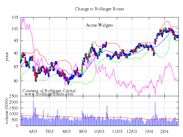
## non-gridded data
[Original Demo](http://gnuplot.sourceforge.net/demo_4.6/scatter.html)
### 1
```ruby
# # Simple demo of scatter data conversion to grid data.
# #
#
# set title "Simple demo of scatter data conversion to grid data"
# unset hidden3d
# set ticslevel 0.5
# set view 60,30
# set autoscale
# set parametric
# set style data points
# set xlabel "data style point - no dgrid"
# set key box
# splot "hemisphr.dat"
Numo.gnuplot do
set title:"Simple demo of scatter data conversion to grid data"
unset :hidden3d
set ticslevel:0.5
set view:[60,30]
set :autoscale
set :parametric
set :style, :data, :points
set xlabel:"data style point - no dgrid"
set :key, :box
splot "\"hemisphr.dat\""
end
```
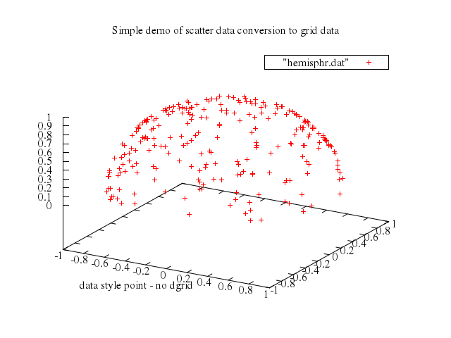
### 2
```ruby
# set dgrid3d 10,10,1
# set xlabel " data style lines, dgrid3d 10,10,1"
# set style data lines
# splot "hemisphr.dat"
Numo.gnuplot do
set dgrid3d:[10,10,1]
set xlabel:" data style lines, dgrid3d 10,10,1"
set :style, :data, :lines
splot "\"hemisphr.dat\""
end
```
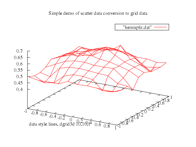
### 3
```ruby
# set dgrid3d ,,4
# set xlabel " data style lines, dgrid3d ,,4 "
# set style data lines
# splot "hemisphr.dat"
Numo.gnuplot do
set dgrid3d:",,4"
set xlabel:" data style lines, dgrid3d ,,4 "
set :style, :data, :lines
splot "\"hemisphr.dat\""
end
```
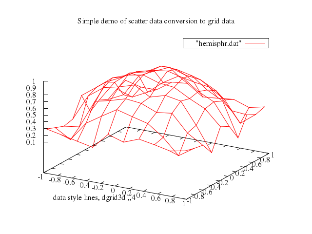
### 4
```ruby
# set dgrid3d ,,16
# set xlabel " data style lines, dgrid3d ,,16"
# set style data lines
# splot "hemisphr.dat"
Numo.gnuplot do
set dgrid3d:",,16"
set xlabel:" data style lines, dgrid3d ,,16"
set :style, :data, :lines
splot "\"hemisphr.dat\""
end
```
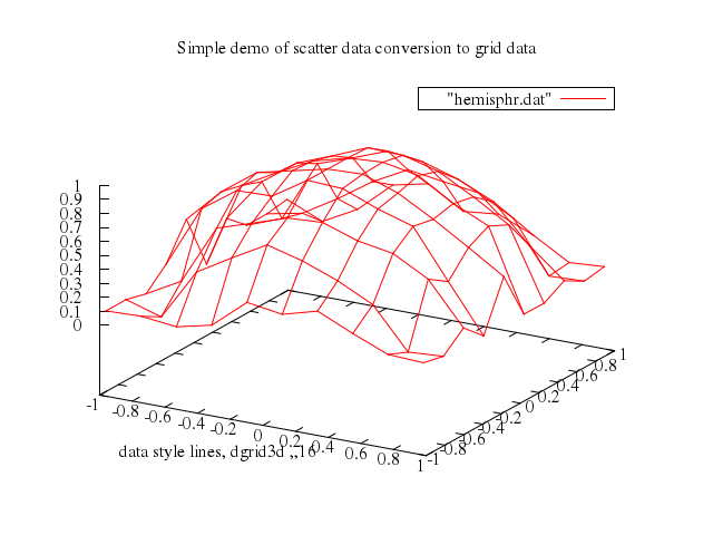
### 5
```ruby
# set contour
# set xlabel "data style lines, dgrid3d ,,16, contour"
# splot "hemisphr.dat"
Numo.gnuplot do
set :contour
set xlabel:"data style lines, dgrid3d ,,16, contour"
splot "\"hemisphr.dat\""
end
```
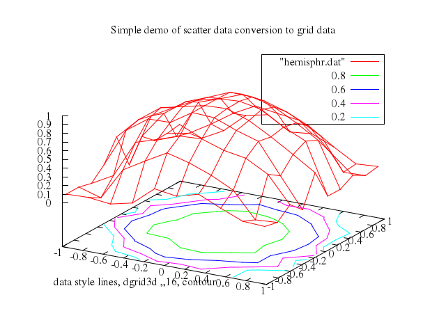
### 6
```ruby
# unset dgrid3d
# set style data points
# set xlabel "data style points, nodgrid3d"
# splot "scatter2.dat"
Numo.gnuplot do
unset :dgrid3d
set :style, :data, :points
set xlabel:"data style points, nodgrid3d"
splot "\"scatter2.dat\""
end
```
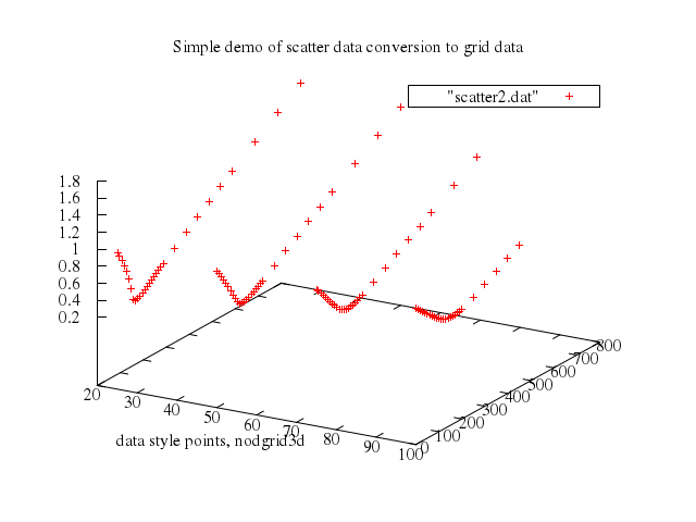
### 7
```ruby
# set key nobox
# set dgrid3d ,,1
# set xlabel "data style lines, dgrid3d ,,1"
# set style data lines
# splot "scatter2.dat"
Numo.gnuplot do
set :key, :nobox
set dgrid3d:",,1"
set xlabel:"data style lines, dgrid3d ,,1"
set :style, :data, :lines
splot "\"scatter2.dat\""
end
```
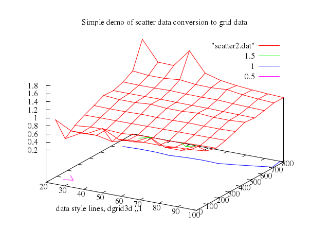
### 8
```ruby
# set dgrid3d ,,4
# set xlabel "data style lines, dgrid3d ,,4"
# set style data lines
# splot "scatter2.dat"
Numo.gnuplot do
set dgrid3d:",,4"
set xlabel:"data style lines, dgrid3d ,,4"
set :style, :data, :lines
splot "\"scatter2.dat\""
end
```
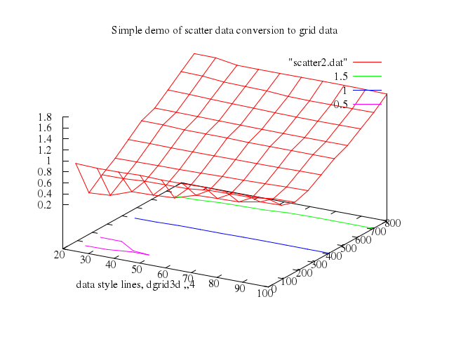
## running averages
[Original Demo](http://gnuplot.sourceforge.net/demo_4.6/running_avg.html)
### 1
```ruby
# # This script demonstrates the use of assignment operators and
# # sequential expression evaluation to track data points as they
# # are read in.
# #
# # We use the '=' and ',' operators to track the running total
# # and previous 5 values of a stream of input data points.
# #
# # Ethan A Merritt - August 2007
# #
# # Define a function to calculate average over previous 5 points
# #
# set title \
# "Demonstrate use of assignment and serial evaluation operators\n" \
# . "to accumulate statistics as successive data lines are read in\n"
# set key invert box center right reverse Left
# set xtics nomirror
# set ytics nomirror
# set border 3
#
# samples(x) = $0 > 4 ? 5 : ($0+1)
# avg5(x) = (shift5(x), (back1+back2+back3+back4+back5)/samples($0))
# shift5(x) = (back5 = back4, back4 = back3, back3 = back2, back2 = back1, back1 = x)
#
# #
# # Initialize a running sum
# #
# init(x) = (back1 = back2 = back3 = back4 = back5 = sum = 0)
#
# #
# # Plot data, running average and cumulative average
# #
#
# datafile = 'silver.dat'
# set xrange [0:57]
#
# set style data linespoints
#
# plot sum = init(0), \
# datafile using 0:2 title 'data' lw 2 lc rgb 'forest-green', \
# '' using 0:(avg5($2)) title "running mean over previous 5 points" pt 7 ps 0.5 lw 1 lc rgb "blue", \
# '' using 0:(sum = sum + $2, sum/($0+1)) title "cumulative mean" pt 1 lw 1 lc rgb "dark-red"
Numo.gnuplot do
set title:"Demonstrate use of assignment and serial evaluation operators\n"+"to accumulate statistics as successive data lines are read in\n"
set :key, :invert, :box, :center, :right, :reverse, :Left
set :xtics, :nomirror
set :ytics, :nomirror
set border:3
run "samples(x) = $0 > 4 ? 5 : ($0+1)"
run "avg5(x) = (shift5(x), (back1+back2+back3+back4+back5)/samples($0))"
run "shift5(x) = (back5 = back4, back4 = back3, back3 = back2, back2 = back1, back1 = x)"
run "init(x) = (back1 = back2 = back3 = back4 = back5 = sum = 0)"
run "datafile = 'silver.dat'"
set xrange:0..57
set :style, :data, :linespoints
plot "sum=init(0)",
[:"datafile", using:[0,2], title:'data', lw:2, lc_rgb:'forest-green'],
["''", using:'0:(avg5($2))', title:"running mean over previous 5 points", pt:7, ps:0.5, lw:1, lc_rgb:"blue"],
["''", using:'0:(sum = sum + $2, sum/($0+1))', title:"cumulative mean", pt:1, lw:1, lc_rgb:"dark-red"]
end
```
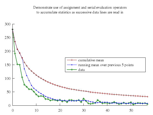
## binning/histograms
[Original Demo](http://gnuplot.sourceforge.net/demo_4.6/smooth.html)
### 1
```ruby
# bin(x, s) = s*int(x/s)
#
# set zeroaxis
#
# # Uniform
# set title "Uniform Distribution"
# set key top right
# set boxwidth 0.05
# plot [-0.1:1.1][-0.4:1.5] "random-points" u 1:(0.25*rand(0)-.35) t '', \
# "" u (bin($1,0.05)):(20/300.) s f t 'smooth frequency' w boxes, \
# "" u 1:(1/300.) s cumul t 'smooth cumulative'
Numo.gnuplot do
run "bin(x, s) = s*int(x/s)"
set :zeroaxis
set title:"Uniform Distribution"
set :key, :top, :right
set boxwidth:0.05
plot -0.1..1.1, -0.4..1.5,
["\"random-points\"", u:'1:(0.25*rand(0)-.35)', t:''],
["\"\"", u:'(bin($1,0.05)):(20/300.)', s:true, f:true, t:'smooth frequency', w:"boxes"],
["\"\"", u:'1:(1/300.)', s:"cumul", t:'smooth cumulative']
end
```
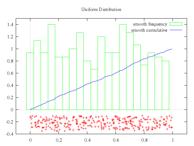
### 2
```ruby
# # Normal
# set title "Normal Distribution"
# set key top left
# set boxwidth 0.05
# plot "random-points" u 2:(0.25*rand(0)-.35) t '', \
# "" u (bin($2,0.05)):(20/300.) s f t 'smooth frequency' w boxes, \
# "" u 2:(1/300.) s cumul t 'smooth cumulative'
Numo.gnuplot do
set title:"Normal Distribution"
set :key, :top, :left
set boxwidth:0.05
plot ["\"random-points\"", u:'2:(0.25*rand(0)-.35)', t:''],
["\"\"", u:'(bin($2,0.05)):(20/300.)', s:true, f:true, t:'smooth frequency', w:"boxes"],
["\"\"", u:'2:(1/300.)', s:"cumul", t:'smooth cumulative']
end
```
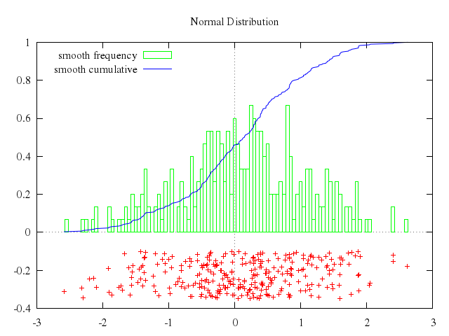
### 3
```ruby
# # Lognormal
# set title "Lognormal Distribution"
# set key top right
# set boxwidth 0.1
# plot [0:] "random-points" u 3:(0.25*rand(0)-.35) t '', \
# "" u (bin($3,0.1)):(10/300.) s f t 'smooth frequency' w boxes, \
# "" u 3:(1/300.) s cumul t 'smooth cumulative'
Numo.gnuplot do
set title:"Lognormal Distribution"
set :key, :top, :right
set boxwidth:0.1
plot "[0:]",
["\"random-points\"", u:'3:(0.25*rand(0)-.35)', t:''],
["\"\"", u:'(bin($3,0.1)):(10/300.)', s:true, f:true, t:'smooth frequency', w:"boxes"],
["\"\"", u:'3:(1/300.)', s:"cumul", t:'smooth cumulative']
end
```
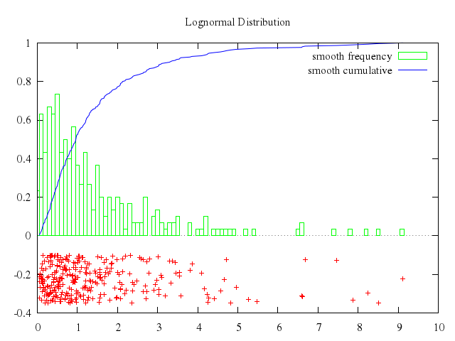
### 4
```ruby
# # Mixed
# set title "Mixed Distribution (Lognormal with shifted Gaussian)"
# set key top right
# set boxwidth 0.1
# plot "random-points" u 4:(0.25*rand(0)-.35) t '', \
# "" u (bin($4,0.1)):(10/300.) s f t 'smooth frequency' w boxes, \
# "" u 4:(1/300.) s cumul t 'smooth cumulative'
Numo.gnuplot do
set title:"Mixed Distribution (Lognormal with shifted Gaussian)"
set :key, :top, :right
set boxwidth:0.1
plot ["\"random-points\"", u:'4:(0.25*rand(0)-.35)', t:''],
["\"\"", u:'(bin($4,0.1)):(10/300.)', s:true, f:true, t:'smooth frequency', w:"boxes"],
["\"\"", u:'4:(1/300.)', s:"cumul", t:'smooth cumulative']
end
```
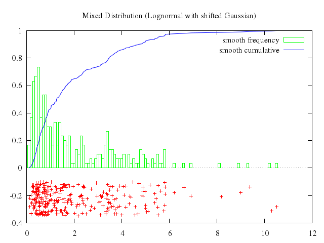
## 2D and 3D heat maps
[Original Demo](http://gnuplot.sourceforge.net/demo_4.6/heatmaps.html)
### 1
```ruby
# # Two ways of generating a 2D heat map from ascii data
# #
#
# set title "Heat Map generated from a file containing Z values only"
# unset key
# set tic scale 0
#
# # Color runs from white to green
# set palette rgbformula -7,2,-7
# set cbrange [0:5]
# set cblabel "Score"
# unset cbtics
#
# set xrange [-0.5:4.5]
# set yrange [-0.5:4.5]
#
# set view map
# splot '-' matrix with image
# 5 4 3 1 0
# 2 2 0 0 1
# 0 0 0 1 0
# 0 0 0 2 3
# 0 1 2 4 3
# e
#
# set title "Heat Map generated by 'plot' from a stream of XYZ values"\
# ."\nNB: Rows must be separated by blank lines!"
Numo.gnuplot do
set title:"Heat Map generated from a file containing Z values only"
unset :key
set :tic, :scale, 0
set :palette, rgbformula:[-7,2,-7]
set cbrange:0..5
set cblabel:"Score"
unset :cbtics
set xrange:-0.5..4.5
set yrange:-0.5..4.5
set view:'map'
run < <&{x@_0^{-3/2}y}> holds space for"
# set label 7 at -0.45, 0.5
# set label 7 "<{{/=20 B}ig}> <{x@_0^{-3/2}y}>"
#
# set label 8 at -0.9, -0.2
# set label 8 "Overprint\n(v should be centred over d)" tc lt 3
# set label 9 at -0.85, -0.4
# set label 9 " ~{abcdefg}{0.8v}"
#
# set label 10 at -.40, 0.35
# set label 10 "UTF-8 encoding does not require Symbol font:" tc lt 3
# set label 11 at -.30, 0.2
# set label 11 "{/*1.5 ∫@_{/=9.6 0}^{/=12 ∞}} {e^{-{μ}^2/2} d}{μ=(π/2)^{1/2}}"
#
# set label 21 at 0.5, -.1
# set label 21 "Left ^{centered} ƒ(αβγδεζ)" left
# set label 22 at 0.5, -.2
# set label 22 "Right ^{centered} ƒ(αβγδεζ)" right
# set label 23 at 0.5, -.3
# set label 23 "Center^{centered} ƒ(αβγδεζ)" center
# #
# set key title " "
# plot sin(x)**2 lt 2 lw 2 title "sin^2(x)"
Numo.gnuplot do
set :termoption, :enhanced
set encoding:"utf8"
set title:"Demo of enhanced text mode using a single UTF-8 encoded font\nThere is another demo that shows how to use a separate Symbol font"
set xrange:-1..1
set yrange:-0.5..1.1
set format_xy:"%.1f"
set :arrow, from:[0.5,-0.5], to:[0.5,0.0], nohead:true
set :label, 1, at:[-0.65,0.95]
set :label, 1, "Superscripts and subscripts:", tc_lt:3
set :label, 3, at:[-0.55,0.85]
set :label, 3, 'A_{j,k} 10^{-2} x@^2_k x@_0^{-3/2}y'
set :label, 5, at:[-0.55,0.7]
set :label, 5, "Space-holders:", tc_lt:3
set :label, 6, at:[-0.45,0.6]
set :label, 6, "<&{{/=20 B}ig}> <&{x@_0^{-3/2}y}> holds space for"
set :label, 7, at:[-0.45,0.5]
set :label, 7, "<{{/=20 B}ig}> <{x@_0^{-3/2}y}>"
set :label, 8, at:[-0.9,-0.2]
set :label, 8, "Overprint\n(v should be centred over d)", tc_lt:3
set :label, 9, at:[-0.85,-0.4]
set :label, 9, " ~{abcdefg}{0.8v}"
set :label, 10, at:[-0.40,0.35]
set :label, 10, "UTF-8 encoding does not require Symbol font:", tc_lt:3
set :label, 11, at:[-0.30,0.2]
set :label, 11, "{/*1.5 ∫@_{/=9.6 0}^{/=12 ∞}} {e^{-{μ}^2/2} d}{μ=(π/2)^{1/2}}"
set :label, 21, at:[0.5,-0.1]
set :label, 21, "Left ^{centered} ƒ(αβγδεζ)", :left
set :label, 22, at:[0.5,-0.2]
set :label, 22, "Right ^{centered} ƒ(αβγδεζ)", :right
set :label, 23, at:[0.5,-0.3]
set :label, 23, "Center^{centered} ƒ(αβγδεζ)", :center
set :key, title:" "
plot "sin(x)**2", lt:2, lw:2, title:"sin^2(x)"
end
```
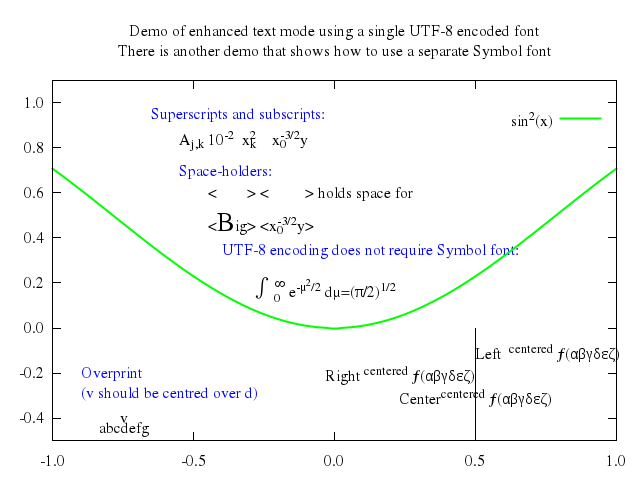
## string data
[Original Demo](http://gnuplot.sourceforge.net/demo_4.6/datastrings.html)
### 1
```ruby
# # Demonstrate features of datastrings patch
# # Ethan A Merritt
# # 08-Mar-2003
# #
# reset
# #
# # Illustrate reading plot labels from column head in datafile
# #
# set title "Auto-labeling plots from text fields in datafile"
# set label 1 "Generate plot labels from first row in each column"
# set label 1 at graph 0.02, 0.85 tc lt 3
# set label 2 "Generate x-axis labels from first column in each row"
# set label 2 at graph 0.02, 0.80 tc lt 3
# set style data linespoints
# set ylabel "mm"
# set yrange [0:200]
# #
# set key autotitle columnhead
# plot 'ctg-y2.dat' using 2:xticlabel(1) index 2, \
# '' using 2 index 3
Numo.gnuplot do
reset
set title:"Auto-labeling plots from text fields in datafile"
set :label, 1, "Generate plot labels from first row in each column"
set :label, 1, at_graph:[0.02,0.85], tc_lt:3
set :label, 2, "Generate x-axis labels from first column in each row"
set :label, 2, at_graph:[0.02,0.80], tc_lt:3
set :style, :data, :linespoints
set ylabel:"mm"
set yrange:0..200
set :key, autotitle:"columnhead"
plot ["'ctg-y2.dat'", using:'2:xticlabel(1)', index:2],
["''", using:2, index:3]
end
```
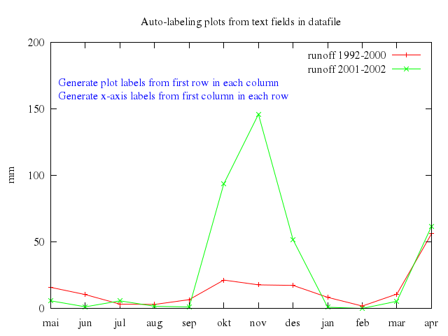
### 2
```ruby
# # Illustrate reading xtic axis labels from the datafile
# #
# reset
# set title "Read tic labels from a datafile column\nAn approximation of Hans Olav Eggestad's categoric plot patch\nusing 'using ($0):2:xticlabels(1)' and 'set style fill solid border -1'"
# set boxwidth 0.3
# set style fill solid 1.000000 border -1
# set bmargin 3
# set pointsize 2
# set yrange [0:180]
# set xrange [-0.5:11.5]
# set ylabel "mm"
# set tics scale 0.0
# set grid y
# set xtics
# #
# set key autotitle columnhead
# plot 'ctg-y2.dat' using ($0-0.2):2 index 0 with boxes title "precipitation 1992-2000", \
# '' using ($0+0.2):2 index 1 with boxes title " 2000-2001", \
# '' using ($0):2 index 2 with linespoints lw 3 title "runoff 1992-2000", \
# '' using ($0):2:xticlabels(1) index 3 with linespoints lw 3 title " 2000-2001"
Numo.gnuplot do
reset
set title:"Read tic labels from a datafile column\nAn approximation of Hans Olav Eggestad's categoric plot patch\nusing 'using ($0):2:xticlabels(1)' and 'set style fill solid border -1'"
set boxwidth:0.3
set :style, fill_solid:1.000000, border:-1
set bmargin:3
set pointsize:2
set yrange:0..180
set xrange:-0.5..11.5
set ylabel:"mm"
set :tics, :scale, 0.0
set grid:"y"
set :xtics
set :key, autotitle:"columnhead"
plot ["'ctg-y2.dat'", using:'($0-0.2):2', index:0, with:"boxes", title:"precipitation 1992-2000"],
["''", using:'($0+0.2):2', index:1, with:"boxes", title:" 2000-2001"],
["''", using:'($0):2', index:2, with:"linespoints", lw:3, title:"runoff 1992-2000"],
["''", using:'($0):2:xticlabels(1)', index:3, with:"linespoints", lw:3, title:" 2000-2001"]
end
```
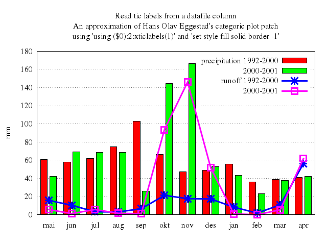
### 3
```ruby
# set title "Same plot using x2ticlabels also"
# set x2tics
# plot 'ctg-y2.dat' using ($0-0.2):2 index 0 with boxes title "precipitation 1992-2000", \
# '' using ($0+0.2):2 index 1 with boxes title " 2000-2001", \
# '' using ($0):2 index 2 with linespoints lw 3 title "runoff 1992-2000", \
# '' using ($0):2:x2ticlabels(1) index 3 with linespoints lw 3 title " 2000-2001"
Numo.gnuplot do
set title:"Same plot using x2ticlabels also"
set :x2tics
plot ["'ctg-y2.dat'", using:'($0-0.2):2', index:0, with:"boxes", title:"precipitation 1992-2000"],
["''", using:'($0+0.2):2', index:1, with:"boxes", title:" 2000-2001"],
["''", using:'($0):2', index:2, with:"linespoints", lw:3, title:"runoff 1992-2000"],
["''", using:'($0):2:x2ticlabels(1)', index:3, with:"linespoints", lw:3, title:" 2000-2001"]
end
```
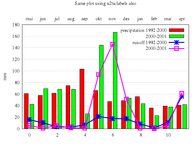
### 4
```ruby
# set title "Plot from table format (titles taken from column headers)"
# unset x2tics
# plot 'table.dat' using ($0-0.2):2 title column(2) with boxes, \
# '' using ($0+0.2):3 title column(3) with boxes, \
# '' using ($0):4 title column(4) with linespoints, \
# '' using ($0):5:xtic(1) title column(5) with linespoints
Numo.gnuplot do
set title:"Plot from table format (titles taken from column headers)"
unset :x2tics
plot ["'table.dat'", using:'($0-0.2):2', title_nq:'column(2)', with:"boxes"],
["''", using:'($0+0.2):3', title_nq:'column(3)', with:"boxes"],
["''", using:'($0):4', title_nq:'column(4)', with:"linespoints"],
["''", using:'($0):5:xtic(1)', title_nq:'column(5)', with:"linespoints"]
end
```
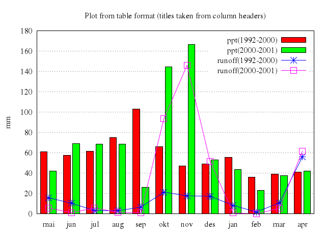
### 5
```ruby
# set title "Plot actual y-value as a label"
# plot 'table.dat' using 0:2:xtic(1) title columnhead with boxes, \
# '' using 0:2:2 with labels center offset 0,1 notitle
Numo.gnuplot do
set title:"Plot actual y-value as a label"
plot ["'table.dat'", using:'0:2:xtic(1)', title_nq:'columnhead', with:"boxes"],
["''", using:[0,2,2], with:"labels", center:true, offset:0],
["1", :notitle]
end
```
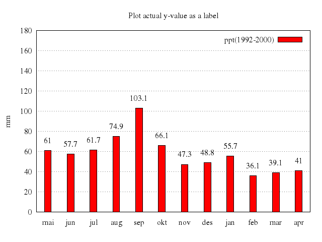
### 6
```ruby
# # Now show the plot with labels options
# #
# reset
#
# set title "Read labels from a datafile column\nHere the 'plot with labels' command generates a\nC-alpha trace of retro-GCN4 peptide"
# set size square
# unset xtics
# unset ytics
# set border 3
# set xlabel "X--->"
# set ylabel "Z--->"
# set key bottom right
# #
# plot 'labelplot.pdb' using 7:9 with lines notitle, \
# '' using 7:9:4 with labels tc lt 3 font "Helvetica,10" notitle
Numo.gnuplot do
reset
set title:"Read labels from a datafile column\nHere the 'plot with labels' command generates a\nC-alpha trace of retro-GCN4 peptide"
set size:"square"
unset :xtics
unset :ytics
set border:3
set xlabel:"X--->"
set ylabel:"Z--->"
set :key, :bottom, :right
plot ["'labelplot.pdb'", using:[7,9], with:"lines", notitle:true],
["''", using:[7,9,4], with:"labels", tc_lt:3, font:"Helvetica,10", notitle:true]
end
```
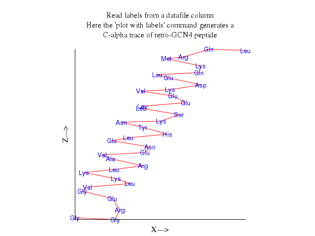
### 7
```ruby
# # '' using 7:9 with points notitle ps 5 lt -1
# #
# reset
#
# set title "3D version generated by splot\n(sorry, the axis scales are distorted)"
# set zrange [-15:15]
#
# set view 70,210, 1.0,1.7
# set ticslevel 0.0
#
# splot 'labelplot.pdb' using 7:8:9 with lines notitle, \
# '' using 7:8:9:4 with labels left offset 1,0 point \
# ps 2 pt 1 tc lt 3 font "Helvetica,10" notitle
Numo.gnuplot do
reset
set title:"3D version generated by splot\n(sorry, the axis scales are distorted)"
set zrange:-15..15
set view:[70,210,1.0,1.7]
set ticslevel:0.0
splot ["'labelplot.pdb'", using:[7,8,9], with:"lines", notitle:true],
["''", using:[7,8,9,4], with:"labels", left:true, offset:1],
["0", point_ps:2, pt:1, tc_lt:3, font:"Helvetica,10", notitle:true]
end
```
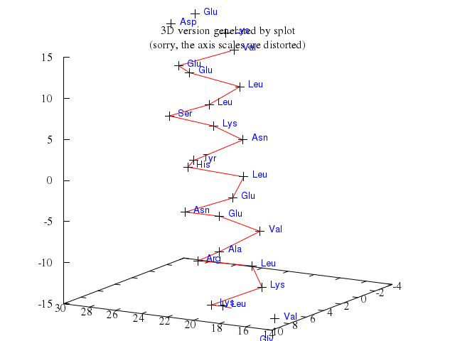
## variable font size
[Original Demo](http://gnuplot.sourceforge.net/demo_4.6/cities.html)
### 1
```ruby
# # Demonstrates how to derive variable font size from a data file column.
# #
# # If you are viewing this via the HTML canvas terminal, be sure to toggle
# # the font scaling icon so that the fonts change size as you zoom in.
# #
# Scale(size) = 0.25*sqrt(sqrt(column(size)))
# CityName(String,Size) = sprintf("{/=%d %s}", Scale(Size), stringcolumn(String))
#
# set termoption enhanced
# set encoding utf8
# unset xtics
# unset ytics
# unset key
# set border 0
# set size square
# set datafile separator "\t"
# plot 'cities.dat' using 5:4:($3 < 5000 ? "-" : CityName(1,3)) with labels
Numo.gnuplot do
run "Scale(size) = 0.25*sqrt(sqrt(column(size)))"
run "CityName(String,Size) = sprintf(\"{/=%d %s}\", Scale(Size), stringcolumn(String))"
set :termoption, :enhanced
set encoding:"utf8"
unset :xtics
unset :ytics
unset :key
set border:0
set size:"square"
set :datafile, :separator, "\t"
plot "'cities.dat'", using:'5:4:($3 < 5000 ? "-" : CityName(1,3))', with:"labels"
end
```
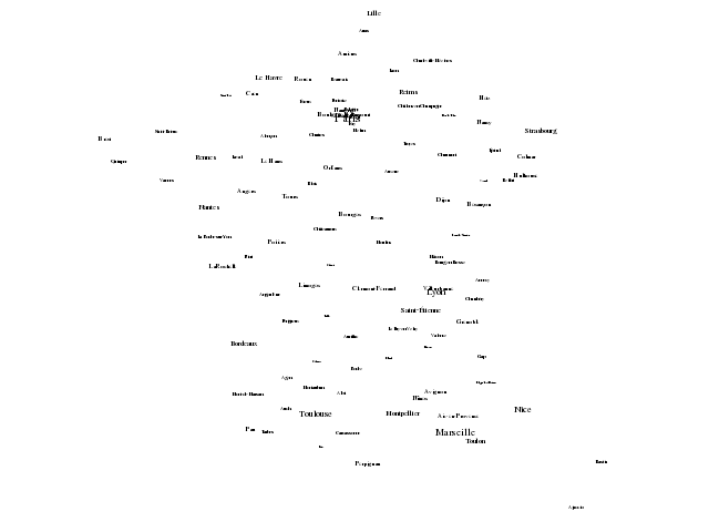
## string variables
[Original Demo](http://gnuplot.sourceforge.net/demo_4.6/stringvar.html)
### 1
```ruby
# # Miscellaneous neat things you can do using the string variables code
# #
# set print "stringvar.tmp"
# print ""
# print "Exercise substring handling"
# print ""
# beg = 2
# end = 4
# print "beg = ",beg," end = ",end
# foo = "ABCDEF"
# print "foo = ",foo
# print "foo[3:5] = ",foo[3:5]
# print "foo[1:1] = ",foo[1:1]
# print "foo[5:3] = ",foo[5:3]
# print "foo[beg:end] = ",foo[beg:end]
# print "foo[end:beg] = ",foo[end:beg]
# print "foo[5:] = ",foo[5:]
# print "foo[5:*] = ",foo[5:*]
# print "foo[:] = ",foo[:]
# print "foo[*:*] = ",foo[*:*]
# print "foo.foo[2:2] = ",foo.foo[2:2]
# print "(foo.foo)[2:2]= ",(foo.foo)[2:2]
# print ""
# unset print
#
# set label 1 system("cat stringvar.tmp") at graph 0.1, graph 0.9
# unset xtics
# unset ytics
# set yrange [0:1]
# plot 0
Numo.gnuplot do
run <($3+$1/50.)) ? "Up" : "Dn" ) with labels \
# title 'plot using 1:2:( ($3>$2) ? "Up" : "Dn" ) with labels'
Numo.gnuplot do
set xrange:0..1
set yrange:0..1
set title:"Constant string expressions as plot symbols"
set xrange:250..500
set auto:"y"
set :style, :data, :lines
plot ["'silver.dat'", u:'1:2:($3+$1/50.)', w:'filledcurves above', title:'Above'],
["''", u:'1:2:($3+$1/50.)', w:'filledcurves below', title:'Below'],
["''", u:[1,2], lt:-1, lw:0.5, notitle:true],
["''", u:'1:($3+$1/50.)', lt:3, lw:0.5, notitle:true],
["''", using:'1:2:( ($2>($3+$1/50.)) ? "Up" : "Dn" )', with:"labels", title:'plot using 1:2:( ($3>$2) ? "Up" : "Dn" ) with labels']
end
```
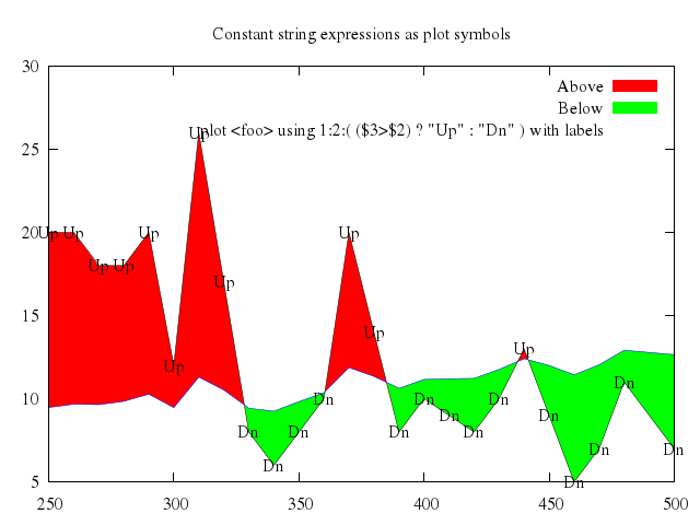
### 5
```ruby
# plot 'silver.dat' \
# u 1:2 lt -1 lw 0.5 notitle, \
# '' u 1:($3+$1/50.) lt 3 lw 0.5 notitle, \
# '' using 1:2:( ($2>($3+$1/50.)) ? "J" : "D" ) with labels font "WingDings,28"\
# title 'Same thing using character glyphs from WingDings font'
Numo.gnuplot do
plot ["'silver.dat'", u:[1,2], lt:-1, lw:0.5, notitle:true],
["''", u:'1:($3+$1/50.)', lt:3, lw:0.5, notitle:true],
["''", using:'1:2:( ($2>($3+$1/50.)) ? "J" : "D" )', with:"labels", font:"WingDings,28", title:'Same thing using character glyphs from WingDings font']
end
```
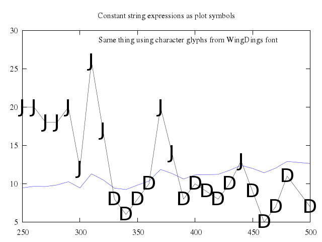
### 6
```ruby
# reset
# set title "String-valued functions to generate datafile names"
# set key title 'file(i) = sprintf("%1d.dat",i); N=2; M=3'
# set key left width 25 Left reverse
# N = 2
# M = 3
# file(i) = sprintf("%1d.dat",i)
# plot 5*sin(x)/x, file(N), file(M)
Numo.gnuplot do
reset
set title:"String-valued functions to generate datafile names"
set :key, title:'file(i) = sprintf("%1d.dat",i); N=2; M=3'
set :key, :left, width:25, Left:true, reverse:true
run "N = 2"
run "M = 3"
run "file(i) = sprintf(\"%1d.dat\",i)"
plot "5*sin(x)/x",
"file(N)",
"file(M)"
end
```
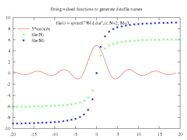
### 7
```ruby
# reset
# fmt = '%Y-%m-%d %H:%M:%S'
# time_str = '2005-05-09 19:44:12'
# seconds = strptime(fmt, time_str)
# time_str2 = strftime(fmt, seconds+10.)
# print ''
# print 'time_str = "', time_str, '"'
# print '-> seconds = ', seconds
# print ' seconds + 10. = ', seconds+10.
# print '-> time_str2 = "', time_str2, '"'
# #
# print ""
# #
# set xdata time
# set key inside left
# #set format x '%Y-%m-%d'
# fmt = "%d/%m/%y\t%H%M"
# print "read_time(fmt, c) =" \
# . " strptime(fmt, stringcolumn(c).' '.stringcolumn(c+1))"
# read_time(fmt, c) = strptime(fmt, stringcolumn(c).' '.stringcolumn(c+1))
# plot 'timedat.dat' using (read_time(fmt,1)):3 with histeps, \
# 'timedat.dat' using (read_time(fmt,1)):($3-0.01):2 with labels title ''
Numo.gnuplot do
reset
run "fmt = '%Y-%m-%d %H:%M:%S'"
run "time_str = '2005-05-09 19:44:12'"
run "seconds = strptime(fmt, time_str)"
run "time_str2 = strftime(fmt, seconds+10.)"
set :xdata, :time
set :key, :inside, :left
run "fmt = \"%d/%m/%y\\t%H%M\""
run "read_time(fmt, c) = strptime(fmt, stringcolumn(c).' '.stringcolumn(c+1))"
plot ["'timedat.dat'", using:'(read_time(fmt,1)):3', with:"histeps"],
["'timedat.dat'", using:'(read_time(fmt,1)):($3-0.01):2', with:"labels", title:'']
end
```
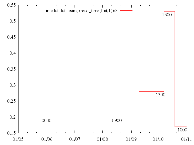
## plot key
[Original Demo](http://gnuplot.sourceforge.net/demo_4.6/key.html)
### 1
```ruby
# # Illustration of key positioning commands and concept.
# #
# # Dan Sebald, 7 nov 2004
# #
# set key default
# set key box
# set key samplen .2
#
# set multiplot layout 3,3
# set key ins vert
# set key left top
# set title "Key (ins vert left top)"
# plot x,-x
# set key center top
# set title "Key (ins vert center top)"
# replot
# set key right
# set title "Key (ins vert right top)"
# replot
# set key center left
# set title "Key (ins vert center left)"
# replot
# set key cent
# set title "Key (inside vertical center)"
# replot
# set key right
# set title "Key (ins vert cent right)"
# replot
# set key bottom left
# set title "Key (ins vert bot left)"
# replot
# set key bot center
# set title "Key (ins vert bot center)"
# replot
# set key right
# set title "Key (ins vert bot right)"
# replot
# unset multiplot
Numo.gnuplot do
set :key, :default
set :key, :box
set :key, samplen:0.2
set :multiplot, layout:[3,3]
set :key, :ins, :vert
set :key, :left, :top
set title:"Key (ins vert left top)"
plot "x",
"-x"
set :key, :center, :top
set title:"Key (ins vert center top)"
replot
set :key, :right
set title:"Key (ins vert right top)"
replot
set :key, :center, :left
set title:"Key (ins vert center left)"
replot
set :key, :cent
set title:"Key (inside vertical center)"
replot
set :key, :right
set title:"Key (ins vert cent right)"
replot
set :key, :bottom, :left
set title:"Key (ins vert bot left)"
replot
set :key, :bot, :center
set title:"Key (ins vert bot center)"
replot
set :key, :right
set title:"Key (ins vert bot right)"
replot
unset :multiplot
end
```
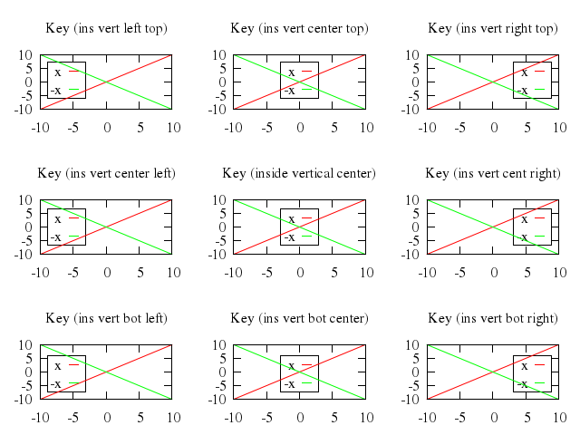
### 2
```ruby
# set multiplot layout 3,3
# set key horiz
# set key left top
# set title "Key (ins horiz left top)"
# replot
# set key center top
# set title "Key (ins horiz center top)"
# replot
# set key right
# set title "Key (ins horiz right top)"
# replot
# set key center left
# set title "Key (ins horiz center left)"
# replot
# set key cent
# set title "Key (inside horizontal center)"
# replot
# set key right
# set title "Key (ins horiz cent right)"
# replot
# set key bottom left
# set title "Key (ins horiz bot left)"
# replot
# set key bot center
# set title "Key (ins horiz bot center)"
# replot
# set key right
# set title "Key (ins horiz bot right)"
# replot
# unset multiplot
Numo.gnuplot do
set :multiplot, layout:[3,3]
set :key, :horiz
set :key, :left, :top
set title:"Key (ins horiz left top)"
replot
set :key, :center, :top
set title:"Key (ins horiz center top)"
replot
set :key, :right
set title:"Key (ins horiz right top)"
replot
set :key, :center, :left
set title:"Key (ins horiz center left)"
replot
set :key, :cent
set title:"Key (inside horizontal center)"
replot
set :key, :right
set title:"Key (ins horiz cent right)"
replot
set :key, :bottom, :left
set title:"Key (ins horiz bot left)"
replot
set :key, :bot, :center
set title:"Key (ins horiz bot center)"
replot
set :key, :right
set title:"Key (ins horiz bot right)"
replot
unset :multiplot
end
```
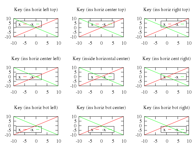
### 3
```ruby
# set multiplot layout 3,3
# set key out vert
# set key left top
# set title "Key (out vert left top)"
# replot
# set key center top
# set title "Key (out vert center top)"
# replot
# set key right
# set title "Key (out vert right top)"
# replot
# set key center left
# set title "Key (out vert center left)"
# replot
# set key cent
# set title "Key (outside vertical center)"
# replot
# set key right
# set title "Key (out vert cent right)"
# replot
# set key bottom left
# set title "Key (out vert bot left)"
# replot
# set key bot center
# set title "Key (out vert bot center)"
# replot
# set key right
# set title "Key (out vert bot right)"
# replot
# unset multiplot
Numo.gnuplot do
set :multiplot, layout:[3,3]
set :key, :out, :vert
set :key, :left, :top
set title:"Key (out vert left top)"
replot
set :key, :center, :top
set title:"Key (out vert center top)"
replot
set :key, :right
set title:"Key (out vert right top)"
replot
set :key, :center, :left
set title:"Key (out vert center left)"
replot
set :key, :cent
set title:"Key (outside vertical center)"
replot
set :key, :right
set title:"Key (out vert cent right)"
replot
set :key, :bottom, :left
set title:"Key (out vert bot left)"
replot
set :key, :bot, :center
set title:"Key (out vert bot center)"
replot
set :key, :right
set title:"Key (out vert bot right)"
replot
unset :multiplot
end
```
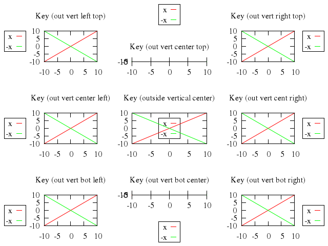
### 4
```ruby
# set multiplot layout 3,3
# set key horiz
# set key left top
# set title "Key (out horiz left top)"
# replot
# set key center top
# set title "Key (out horiz center top)"
# replot
# set key right
# set title "Key (out horiz right top)"
# replot
# set key center left
# set title "Key (out horiz center left)"
# replot
# set key cent
# set title "Key (outside horizontal center)"
# replot
# set key right
# set title "Key (out horiz cent right)"
# replot
# set key bottom left
# set title "Key (out horiz bot left)"
# replot
# set key bot center
# set title "Key (out horiz bot center)"
# replot
# set key right
# set title "Key (out horiz bot right)"
# replot
# unset multiplot
Numo.gnuplot do
set :multiplot, layout:[3,3]
set :key, :horiz
set :key, :left, :top
set title:"Key (out horiz left top)"
replot
set :key, :center, :top
set title:"Key (out horiz center top)"
replot
set :key, :right
set title:"Key (out horiz right top)"
replot
set :key, :center, :left
set title:"Key (out horiz center left)"
replot
set :key, :cent
set title:"Key (outside horizontal center)"
replot
set :key, :right
set title:"Key (out horiz cent right)"
replot
set :key, :bottom, :left
set title:"Key (out horiz bot left)"
replot
set :key, :bot, :center
set title:"Key (out horiz bot center)"
replot
set :key, :right
set title:"Key (out horiz bot right)"
replot
unset :multiplot
end
```
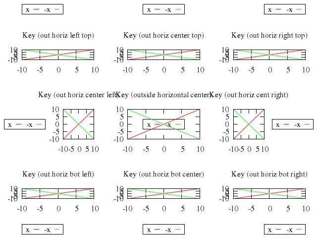
### 5
```ruby
# set multiplot layout 3,3
# set key vert
# set arrow 1 from -3,0 to 3,0 nohead lt -1
# set arrow 2 from 0,-3 to 0,3 nohead lt -1
# set key at 0,0 left top
# set title "Key ( vert left top)"
# replot
# set key at 0,0 center top
# set title "Key ( vert center top)"
# replot
# set key at 0,0 right
# set title "Key ( vert right top)"
# replot
# set key at 0,0 center left
# set title "Key ( vert center left)"
# replot
# set key at 0,0 cent
# set title "Key ( vertical center)"
# replot
# set key at 0,0 right
# set title "Key ( vert cent right)"
# replot
# set key at 0,0 bottom left
# set title "Key ( vert bot left)"
# replot
# set key at 0,0 bot center
# set title "Key ( vert bot center)"
# replot
# set key at 0,0 right
# set title "Key ( vert bot right)"
# replot
# unset multiplot
Numo.gnuplot do
set :multiplot, layout:[3,3]
set :key, :vert
set :arrow, 1, from:[-3,0], to:[3,0], nohead:true, lt:-1
set :arrow, 2, from:[0,-3], to:[0,3], nohead:true, lt:-1
set :key, at:[0,0], left:true, top:true
set title:"Key ( vert left top)"
replot
set :key, at:[0,0], center:true, top:true
set title:"Key ( vert center top)"
replot
set :key, at:[0,0], right:true
set title:"Key ( vert right top)"
replot
set :key, at:[0,0], center:true, left:true
set title:"Key ( vert center left)"
replot
set :key, at:[0,0], cent:true
set title:"Key ( vertical center)"
replot
set :key, at:[0,0], right:true
set title:"Key ( vert cent right)"
replot
set :key, at:[0,0], bottom:true, left:true
set title:"Key ( vert bot left)"
replot
set :key, at:[0,0], bot:true, center:true
set title:"Key ( vert bot center)"
replot
set :key, at:[0,0], right:true
set title:"Key ( vert bot right)"
replot
unset :multiplot
end
```
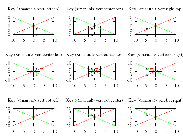
### 6
```ruby
# set multiplot layout 3,3
# set key horiz
# set arrow 1 from -3,0 to 3,0 nohead lt -1
# set arrow 2 from 0,-3 to 0,3 nohead lt -1
# set key at 0,0 left top
# set title "Key ( horiz left top)"
# set xrange [-5:15]
# replot
# set key at 0,0 center top
# set title "Key ( horiz center top)"
# set xrange [-10:10]
# replot
# set key at 0,0 right
# set title "Key ( horiz right top)"
# set xrange [-15:5]
# replot
# set key at 0,0 center left
# set title "Key ( horiz center left)"
# set xrange [-5:15]
# replot
# set key at 0,0 cent
# set title "Key ( horizontal center)"
# set xrange [-10:10]
# replot
# set key at 0,0 right
# set title "Key ( horiz cent right)"
# set xrange [-15:5]
# replot
# set key at 0,0 bottom left
# set title "Key ( horiz bot left)"
# set xrange [-5:15]
# replot
# set key at 0,0 bot center
# set title "Key ( horiz bot center)"
# set xrange [-10:10]
# replot
# set key at 0,0 right
# set title "Key ( horiz bot right)"
# set xrange [-15:5]
# replot
# unset multiplot
Numo.gnuplot do
set :multiplot, layout:[3,3]
set :key, :horiz
set :arrow, 1, from:[-3,0], to:[3,0], nohead:true, lt:-1
set :arrow, 2, from:[0,-3], to:[0,3], nohead:true, lt:-1
set :key, at:[0,0], left:true, top:true
set title:"Key ( horiz left top)"
set xrange:-5..15
replot
set :key, at:[0,0], center:true, top:true
set title:"Key ( horiz center top)"
set xrange:-10..10
replot
set :key, at:[0,0], right:true
set title:"Key ( horiz right top)"
set xrange:-15..5
replot
set :key, at:[0,0], center:true, left:true
set title:"Key ( horiz center left)"
set xrange:-5..15
replot
set :key, at:[0,0], cent:true
set title:"Key ( horizontal center)"
set xrange:-10..10
replot
set :key, at:[0,0], right:true
set title:"Key ( horiz cent right)"
set xrange:-15..5
replot
set :key, at:[0,0], bottom:true, left:true
set title:"Key ( horiz bot left)"
set xrange:-5..15
replot
set :key, at:[0,0], bot:true, center:true
set title:"Key ( horiz bot center)"
set xrange:-10..10
replot
set :key, at:[0,0], right:true
set title:"Key ( horiz bot right)"
set xrange:-15..5
replot
unset :multiplot
end
```
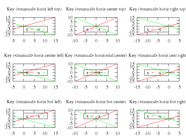
## multiplot layout
[Original Demo](http://gnuplot.sourceforge.net/demo_4.6/layout.html)
### 1
```ruby
# # Gnuplot version 4.1 demo of multiplot
# # auto-layout capability
# #
# set multiplot layout 3, 1 title "Multiplot layout 3, 1" font ",14"
# set tmargin 2
# set title "Plot 1"
# unset key
# plot sin(x)/x
# #
# set title "Plot 2"
# unset key
# plot 'silver.dat' using 1:2 ti 'silver.dat'
# #
# set style histogram columns
# set style fill solid
# set key autotitle column
# set boxwidth 0.8
# set format y " "
# set tics scale 0
# set title "Plot 3"
# plot 'immigration.dat' using 2 with histograms, \
# '' using 7 with histograms , \
# '' using 8 with histograms , \
# '' using 11 with histograms
# #
# unset multiplot
Numo.gnuplot do
set :multiplot, layout:[3,1], title:"Multiplot layout 3, 1", font:",14"
set tmargin:2
set title:"Plot 1"
unset :key
plot "sin(x)/x"
set title:"Plot 2"
unset :key
plot "'silver.dat'", using:[1,2], ti:'silver.dat'
set :style, histogram:"columns"
set :style, :fill_solid
set :key, autotitle:"column"
set boxwidth:0.8
set format_y:" "
set :tics, :scale, 0
set title:"Plot 3"
plot ["'immigration.dat'", using:2, with:"histograms"],
["''", using:7, with:"histograms"],
["''", using:8, with:"histograms"],
["''", using:11, with:"histograms"]
unset :multiplot
end
```
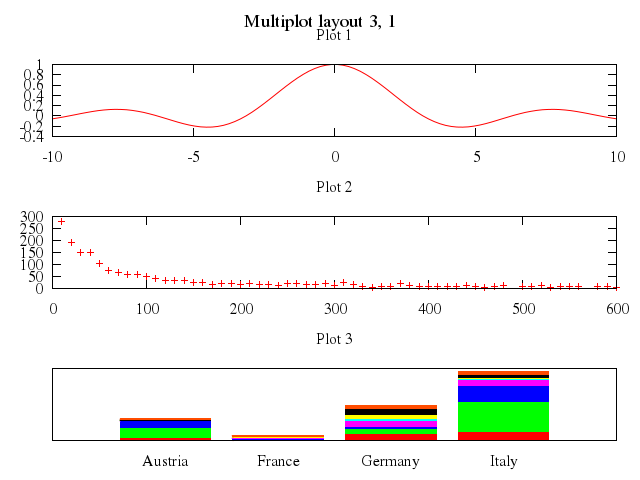
### 2
```ruby
# reset
# set multiplot layout 1,3 title "Multiplot layout 1, 3" font ",14"
# set xtics rotate
# set bmargin 5
# #
# set title "Plot 1"
# unset key
# plot sin(x)/x
# #
# set title "Plot 2"
# unset key
# plot 'silver.dat' using 1:2 ti 'silver.dat'
# #
# set title "Plot 3"
# set style histogram columns
# set style fill solid
# set key autotitle column
# set boxwidth 0.8
# set format y " "
# set tics scale 0
# plot 'immigration.dat' using 2 with histograms , \
# '' using 7 with histograms , \
# '' using 8 with histograms , \
# '' using 11 with histograms
# #
# unset multiplot
Numo.gnuplot do
reset
set :multiplot, layout:[1,3], title:"Multiplot layout 1, 3", font:",14"
set :xtics, :rotate
set bmargin:5
set title:"Plot 1"
unset :key
plot "sin(x)/x"
set title:"Plot 2"
unset :key
plot "'silver.dat'", using:[1,2], ti:'silver.dat'
set title:"Plot 3"
set :style, histogram:"columns"
set :style, :fill_solid
set :key, autotitle:"column"
set boxwidth:0.8
set format_y:" "
set :tics, :scale, 0
plot ["'immigration.dat'", using:2, with:"histograms"],
["''", using:7, with:"histograms"],
["''", using:8, with:"histograms"],
["''", using:11, with:"histograms"]
unset :multiplot
end
```
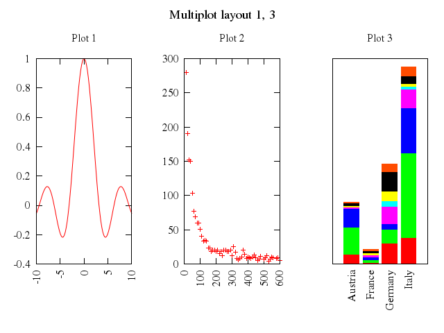
### 3
```ruby
# reset
# set multiplot layout 1,3 title "Same plot with a multi-line title\nshowing adjustment of plot area\n to accommodate it" font ",14"
# set xtics rotate
# set bmargin 5
# #
# set title "Plot 1"
# unset key
# plot sin(x)/x
# #
# set title "Plot 2"
# unset key
# plot 'silver.dat' using 1:2 ti 'silver.dat'
# #
# set title "Plot 3"
# set style histogram columns
# set style fill solid
# set key autotitle column
# set boxwidth 0.8
# set format y " "
# set tics scale 0
# plot 'immigration.dat' using 2 with histograms , \
# '' using 7 with histograms , \
# '' using 8 with histograms , \
# '' using 11 with histograms
# #
# unset multiplot
Numo.gnuplot do
reset
set :multiplot, layout:[1,3], title:"Same plot with a multi-line title\nshowing adjustment of plot area\n to accommodate it", font:",14"
set :xtics, :rotate
set bmargin:5
set title:"Plot 1"
unset :key
plot "sin(x)/x"
set title:"Plot 2"
unset :key
plot "'silver.dat'", using:[1,2], ti:'silver.dat'
set title:"Plot 3"
set :style, histogram:"columns"
set :style, :fill_solid
set :key, autotitle:"column"
set boxwidth:0.8
set format_y:" "
set :tics, :scale, 0
plot ["'immigration.dat'", using:2, with:"histograms"],
["''", using:7, with:"histograms"],
["''", using:8, with:"histograms"],
["''", using:11, with:"histograms"]
unset :multiplot
end
```
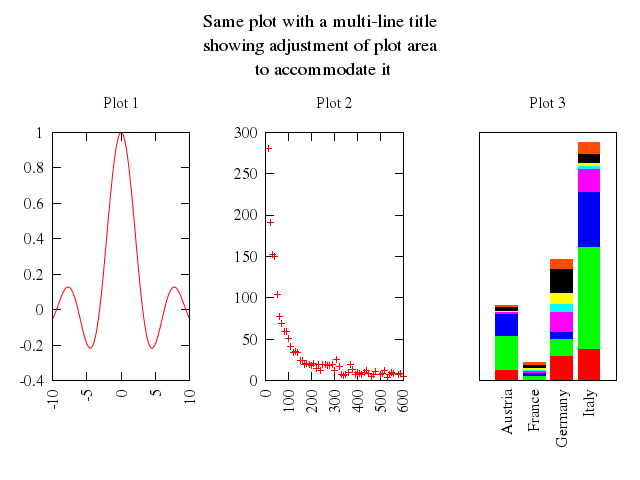
### 4
```ruby
# # Stacked Plot Demo
# #
# # Set top and bottom margins to 0 so that there is no space between plots.
# # Fix left and right margins to make sure that the alignment is perfect.
# # Turn off xtics for all plots except the bottom one.
# # In order to leave room for axis and tic labels underneath, we ask for
# # a 4-plot layout but only use the top 3 slots.
# #
# set tmargin 0
# set bmargin 0
# set lmargin 3
# set rmargin 3
# unset xtics
# unset ytics
#
# set multiplot layout 4,1 title "Auto-layout of stacked plots\n"
#
# set key autotitle column nobox samplen 1 noenhanced
# unset title
# set style data boxes
# set yrange [0 : 800000]
#
# plot 'immigration.dat' using 3 lt 1
# plot 'immigration.dat' using 8 lt 3
# set xtics nomirror
# set tics scale 0 font ",8"
# set xlabel "Immigration to U.S. by Decade"
# plot 'immigration.dat' using 21:xtic(1) lt 4
#
# unset multiplot
Numo.gnuplot do
set tmargin:0
set bmargin:0
set lmargin:3
set rmargin:3
unset :xtics
unset :ytics
set :multiplot, layout:[4,1], title:"Auto-layout of stacked plots\n"
set :key, autotitle:"column", nobox:true, samplen:1, noenhanced:true
unset :title
set :style, :data, :boxes
set yrange:0..800000
plot "'immigration.dat'", using:3, lt:1
plot "'immigration.dat'", using:8, lt:3
set :xtics, :nomirror
set :tics, :scale, 0, font:",8"
set xlabel:"Immigration to U.S. by Decade"
plot "'immigration.dat'", using:'21:xtic(1)', lt:4
unset :multiplot
end
```
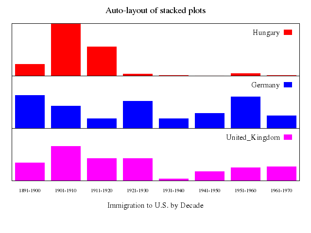
## multiple plots
[Original Demo](http://gnuplot.sourceforge.net/demo_4.6/multiplt.html)
### 1
```ruby
# # GNUPLOT v3.6 beta multiplot script file
# #
# # Second Order System Characteristics
# #
# # D**2 + 2*zeta*wn*D + (wn**2)y = (wn**2)*x
# #
# # x input variable
# # y output variable
# # w frequency ratio (w/wn)
# # wn natural frequency
# # wd damped natural frequency
# # zeta damping ratio
# # mag(w) amplitude response
# # phi(w) phase response
# # wdwn damped natural frequency ratio
# # wnt normalized time
# #
# # Plots:
# # Frequency domain magnitude response
# # phase response
# #
# # Time domain unit step response
# # unit impulse response
# #
# # Created by: W. D. Kirby email: [email protected]
# # Date: 1/18/96
# # Released to the public domain with no warranty of any kind
# #
# reset
# set style function lines
# set size 1.0, 1.0
# set origin 0.0, 0.0
# set multiplot
# set size 0.5,0.5
# set origin 0.0,0.5
# set grid
# unset key
# set angles radians
# set samples 250
# # Plot Magnitude Response
# set title "Second Order System Transfer Function - Magnitude"
# mag(w) = -10*log10( (1-w**2)**2 + 4*(zeta*w)**2)
# set dummy w
# set logscale x
# set xlabel "Frequency (w/wn)"
# set ylabel "Magnitude (dB)" offset 1,0
# set label 1 "Damping =.1,.2,.3,.4,.5,.707,1.0,2.0" at .14,17
# set xrange [.1:10]
# set yrange [-40:20]
# plot \
# zeta=.1,mag(w), \
# zeta=.2,mag(w), \
# zeta=.3,mag(w), \
# zeta=.4,mag(w), \
# zeta=.5,mag(w), \
# zeta=.707,mag(w), \
# zeta=1.0,mag(w), \
# zeta=2.0,mag(w),-6
# # Plot Phase Response
# set size 0.5,0.5
# set origin 0.0,0.0
# set title "Second Order System Transfer Function - Phase"
# set label 1 ""
# set ylabel "Phase (deg)" offset 1,0
# set ytics -180, 30, 0
# set yrange [-180:0]
# tmp(w) = (-180/pi)*atan( 2*zeta*w/(1-w**2) )
# # Fix for atan function wrap problem
# tmp1(w)= w<1?tmp(w):(tmp(w)-180)
# phi(w)=zeta==1?(-2*(180/pi)*atan(w)):tmp1(w)
# plot \
# zeta=.1,phi(w), \
# zeta=.2,phi(w), \
# zeta=.3,phi(w), \
# zeta=.4,phi(w), \
# zeta=.5,phi(w), \
# zeta=.707,phi(w), \
# zeta=1,phi(w), \
# zeta=2.0,phi(w), \
# -90
# # Plot Step Response
# set size 0.5,0.5
# set origin 0.5,0.5
# set dummy wnt
# unset logscale x
# set title "Second Order System - Unit Step Response"
# set ylabel "Amplitude y(wnt)" offset 1,0
# set xlabel "Normalized Time (wnt)"
# set xrange [0:20]
# set xtics 0,5,20
# set yrange [0:2.0]
# set ytics 0, .5, 2.0
# set mytics 5
# set mxtics 10
# wdwn(zeta)=sqrt(1-zeta**2)
# shift(zeta) = atan(wdwn(zeta)/zeta)
# alpha(zeta)=zeta>1?sqrt(zeta**2-1.0):0
# tau1(zeta)=1/(zeta-alpha(zeta))
# tau2(zeta)=1/(zeta+alpha(zeta))
# c1(zeta)=(zeta + alpha(zeta))/(2*alpha(zeta))
# c2(zeta)=c1(zeta)-1
# y1(wnt)=zeta==1?1 - exp(-wnt)*(wnt + 1):0
# y2(wnt)=zeta<1?(1 - (exp(-zeta*wnt)/wdwn(zeta))*sin(wdwn(zeta)*wnt + shift(zeta))):y1(wnt)
# y(wnt)=zeta>1?1-c1(zeta)*exp(-wnt/tau1(zeta))+c2(zeta)*exp(-wnt/tau2(zeta)):y2(wnt)
# plot \
# zeta=.1,y(wnt), \
# zeta=.2,y(wnt), \
# zeta=.3,y(wnt), \
# zeta=.4,y(wnt), \
# zeta=.5,y(wnt), \
# zeta=.707,y(wnt), \
# zeta=1,y(wnt), \
# zeta=2,y(wnt)
# #
# # Plot Impulse Response
# set origin .5,0.
# set title "Second Order System - Unit Impulse Response"
# y(wnt)=exp(-zeta*wnt) * sin(wdwn(zeta)*wnt) / wdwn(zeta)
# set yrange [-1. :1.]
# set ytics -1,.5,1.
# plot \
# zeta=.1,y(wnt), \
# zeta=.2,y(wnt), \
# zeta=.3,y(wnt), \
# zeta=.4,y(wnt), \
# zeta=.5,y(wnt), \
# zeta=.707,y(wnt), \
# zeta=1,y(wnt), \
# zeta=2,y(wnt)
# unset multiplot
Numo.gnuplot do
reset
set :style, :function, :lines
set size:[1.0,1.0]
set origin:[0.0,0.0]
set :multiplot
set size:[0.5,0.5]
set origin:[0.0,0.5]
set :grid
unset :key
set angles:"radians"
set samples:250
set title:"Second Order System Transfer Function - Magnitude"
run "mag(w) = -10*log10( (1-w**2)**2 + 4*(zeta*w)**2)"
set dummy:"w"
set logscale:"x"
set xlabel:"Frequency (w/wn)"
set ylabel:"Magnitude (dB)", offset:[1,0]
set :label, 1, "Damping =.1,.2,.3,.4,.5,.707,1.0,2.0", at:[0.14,17]
set xrange:0.1..10
set yrange:-40..20
plot "zeta=.1",
"mag(w)",
"zeta=.2",
"mag(w)",
"zeta=.3",
"mag(w)",
"zeta=.4",
"mag(w)",
"zeta=.5",
"mag(w)",
"zeta=.707",
"mag(w)",
"zeta=1.0",
"mag(w)",
"zeta=2.0",
"mag(w)",
"-6"
set size:[0.5,0.5]
set origin:[0.0,0.0]
set title:"Second Order System Transfer Function - Phase"
set :label, 1, ""
set ylabel:"Phase (deg)", offset:[1,0]
set ytics:[-180,30,0]
set yrange:-180..0
run "tmp(w) = (-180/pi)*atan( 2*zeta*w/(1-w**2) )"
run "tmp1(w)= w<1?tmp(w):(tmp(w)-180)"
run "phi(w)=zeta==1?(-2*(180/pi)*atan(w)):tmp1(w)"
plot "zeta=.1",
"phi(w)",
"zeta=.2",
"phi(w)",
"zeta=.3",
"phi(w)",
"zeta=.4",
"phi(w)",
"zeta=.5",
"phi(w)",
"zeta=.707",
"phi(w)",
"zeta=1",
"phi(w)",
"zeta=2.0",
"phi(w)",
"-90"
set size:[0.5,0.5]
set origin:[0.5,0.5]
set dummy:"wnt"
unset logscale:"x"
set title:"Second Order System - Unit Step Response"
set ylabel:"Amplitude y(wnt)", offset:[1,0]
set xlabel:"Normalized Time (wnt)"
set xrange:0..20
set xtics:[0,5,20]
set yrange:0..2.0
set ytics:[0,0.5,2.0]
set mytics:5
set mxtics:10
run "wdwn(zeta)=sqrt(1-zeta**2)"
run "shift(zeta) = atan(wdwn(zeta)/zeta)"
run "alpha(zeta)=zeta>1?sqrt(zeta**2-1.0):0"
run "tau1(zeta)=1/(zeta-alpha(zeta))"
run "tau2(zeta)=1/(zeta+alpha(zeta))"
run "c1(zeta)=(zeta + alpha(zeta))/(2*alpha(zeta))"
run "c2(zeta)=c1(zeta)-1"
run "y1(wnt)=zeta==1?1 - exp(-wnt)*(wnt + 1):0"
run "y2(wnt)=zeta<1?(1 - (exp(-zeta*wnt)/wdwn(zeta))*sin(wdwn(zeta)*wnt + shift(zeta))):y1(wnt)"
run "y(wnt)=zeta>1?1-c1(zeta)*exp(-wnt/tau1(zeta))+c2(zeta)*exp(-wnt/tau2(zeta)):y2(wnt)"
plot "zeta=.1",
"y(wnt)",
"zeta=.2",
"y(wnt)",
"zeta=.3",
"y(wnt)",
"zeta=.4",
"y(wnt)",
"zeta=.5",
"y(wnt)",
"zeta=.707",
"y(wnt)",
"zeta=1",
"y(wnt)",
"zeta=2",
"y(wnt)"
set origin:[0.5,0.0]
set title:"Second Order System - Unit Impulse Response"
run "y(wnt)=exp(-zeta*wnt) * sin(wdwn(zeta)*wnt) / wdwn(zeta)"
set yrange:-1.0..1.0
set ytics:[-1,0.5,1.0]
plot "zeta=.1",
"y(wnt)",
"zeta=.2",
"y(wnt)",
"zeta=.3",
"y(wnt)",
"zeta=.4",
"y(wnt)",
"zeta=.5",
"y(wnt)",
"zeta=.707",
"y(wnt)",
"zeta=1",
"y(wnt)",
"zeta=2",
"y(wnt)"
unset :multiplot
end
```
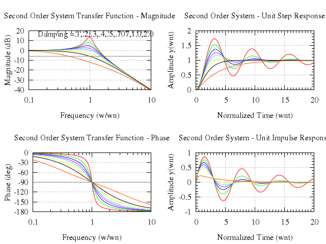
## aligned plots
[Original Demo](http://gnuplot.sourceforge.net/demo_4.6/margins.html)
### 1
```ruby
# # Demonstrate use of 'set {btlr}margin at screen '
# # to pin plot borders to a specific place on the canvas.
# # This allows positioning multiple plots on the page so that their
# # corners line up perfectly.
# #
# # Aug 2006 - Ethan A Merritt
# #
#
# set multiplot title "Demo of placing multiple plots (2D and 3D)\nwith explicit alignment of plot borders"
#
# #
# # First plot (large)
# #
# set lmargin at screen 0.20
# set rmargin at screen 0.85
# set bmargin at screen 0.25
# set tmargin at screen 0.90
#
# set pm3d
# set palette rgbformulae 7, 5, 15
# set view map
# set samples 50, 50
# set isosamples 50, 50
# unset surface
# set xrange [ -15.00 : 15.00 ]
# set yrange [ -15.00 : 15.00 ]
# set zrange [ -0.250 : 1.000 ]
#
# unset xtics
# unset ytics
#
# set key above
#
# splot sin(sqrt(x**2+y**2))/sqrt(x**2+y**2)
#
# unset pm3d
# unset key
#
# #
# # second plot (tall and narrow; at left of main plot)
# #
# set lmargin at screen 0.10
# set rmargin at screen 0.20
#
# set ytics
#
# set parametric
# set dummy u,v
# set view map
#
# f(h) = sin(sqrt(h**2))/sqrt(h**2)
#
# set urange [ -15.00 : 15.00 ]
# set vrange [ -15.00 : 15.00 ]
# set xrange [*:*]
# set surface
#
# splot f(u), u, 0 with lines lc rgb "green"
#
# unset parametric
#
# #
# # third plot (short and wide; at bottom of main plot)
# #
# set lmargin at screen 0.20
# set rmargin at screen 0.85
# set bmargin at screen 0.10
# set tmargin at screen 0.25
#
# set xrange [ -15.00 : 15.00 ]
# set yrange [ * : * ]
# set xtics
# unset ytics
#
# y = 0
# plot sin(sqrt(x**2+y**2))/sqrt(x**2+y**2)
#
# unset multiplot
Numo.gnuplot do
set :multiplot, title:"Demo of placing multiple plots (2D and 3D)\nwith explicit alignment of plot borders"
set :lmargin, :at, screen:0.20
set :rmargin, :at, screen:0.85
set :bmargin, :at, screen:0.25
set :tmargin, :at, screen:0.90
set :pm3d
set :palette, rgbformulae:[7,5,15]
set view:'map'
set samples:[50,50]
set isosamples:[50,50]
unset :surface
set xrange:-15.00..15.00
set yrange:-15.00..15.00
set zrange:-0.250..1.000
unset :xtics
unset :ytics
set :key, "above"
splot "sin(sqrt(x**2+y**2))/sqrt(x**2+y**2)"
unset :pm3d
unset :key
set :lmargin, :at, screen:0.10
set :rmargin, :at, screen:0.20
set :ytics
set :parametric
set dummy:"u,v"
set view:'map'
run "f(h) = sin(sqrt(h**2))/sqrt(h**2)"
set urange:-15.00..15.00
set vrange:-15.00..15.00
set xrange:"[*:*]"
set :surface
splot "f(u)",
"u",
["0", with:"lines", lc_rgb:"green"]
unset :parametric
set :lmargin, :at, screen:0.20
set :rmargin, :at, screen:0.85
set :bmargin, :at, screen:0.10
set :tmargin, :at, screen:0.25
set xrange:-15.00..15.00
set yrange:"[*:*]"
set :xtics
unset :ytics
run "y = 0"
plot "sin(sqrt(x**2+y**2))/sqrt(x**2+y**2)"
unset :multiplot
end
```
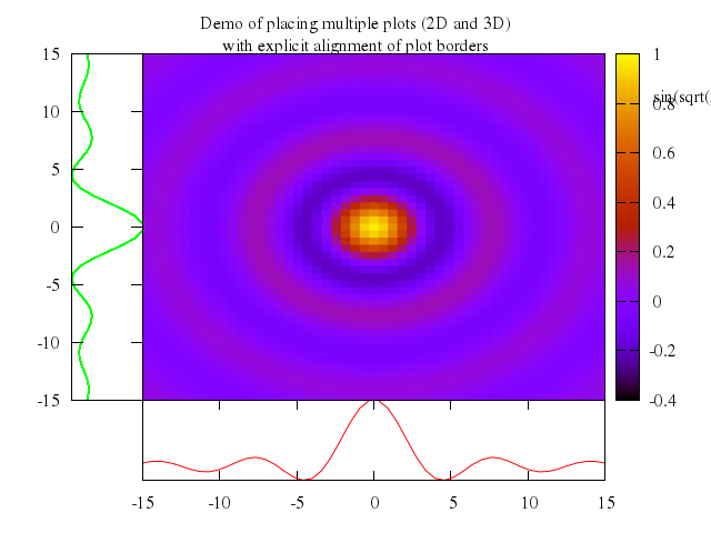
## axis location
[Original Demo](http://gnuplot.sourceforge.net/demo_4.6/ellipse.html)
### 1
```ruby
# # Ethan A Merritt - Feb 2007
# # This demo requires support for 'set object ellipse'
# # Also it uses the file 'random.tmp' created by random.dem
# #
# if ((GPVAL_VERSION == 4.3 || GPVAL_VERSION == 4.2) \
# && (!strstrt(GPVAL_COMPILE_OPTIONS,"+OBJECTS"))) \
# print ">>> Skipping demo <<<\n" ; \
# print "This copy of gnuplot was built without support for placing ellipses\n" ; \
# exit ;
#
# unset key
# set xrange [-8:8]
# set yrange [-8:8]
# set size ratio 1.0
# set zeroaxis
# set border 0
# set xtics axis
# set ytics axis
# set tics scale 0.5
# set format xy ""
#
# set title 'Example of `set object ellipse`'
#
# set object 1 ellipse center 1.5,1.0 size 2.,4. angle 20. front fillstyle empty border -1
# set obj 2 ellipse center 1.5, 1 size 6, 12 angle 20 front fs empty bo 3
#
# A = pi/9.
# plot 'random.tmp' using (1.5 + $1*cos(A)-2.*$2*sin(A)):(1.0 + $1*sin(A)+2.*$2*cos(A)) with dots
Numo.gnuplot do
unset :key
set xrange:-8..8
set yrange:-8..8
set :size, :ratio, 1.0
set :zeroaxis
set border:0
set :xtics, :axis
set :ytics, :axis
set :tics, :scale, 0.5
set format_xy:""
set title:'Example of `set object ellipse`'
set :object, 1, :ellipse, center:[1.5,1.0], size:[2.0,4.0], angle:20.0, front:true, fillstyle:true, empty:true, border:-1
set :obj, 2, :ellipse, center:[1.5,1], size:[6,12], angle:20, front:true, fs:true, empty:true, bo:3
run "A = pi/9."
plot "'random.tmp'", using:'(1.5 + $1*cos(A)-2.*$2*sin(A)):(1.0 + $1*sin(A)+2.*$2*cos(A))', with:"dots"
end
```
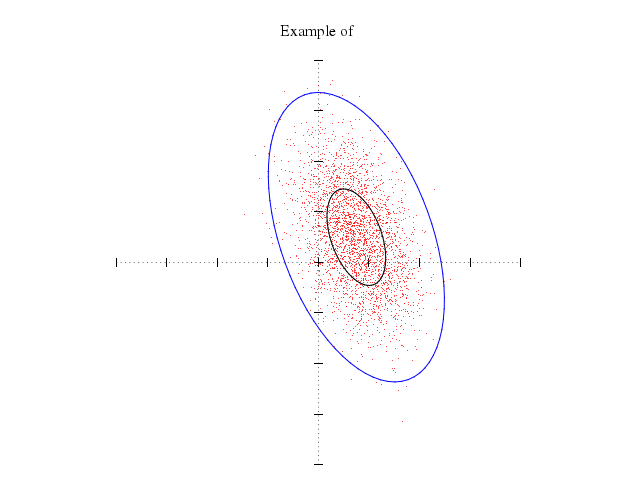
### 2
```ruby
# set title 'Example of range-limited axes and tics'
#
# set tics out scale 0.5
# set xtics 1.0 border rangelimited nomirror
# set ytics 1.0 border rangelimited nomirror
# set format xy "%.0f"
# set border 3
#
# replot
Numo.gnuplot do
set title:'Example of range-limited axes and tics'
set :tics, :out, scale:0.5
set xtics:1.0, border:"rangelimited", nomirror:true
set ytics:1.0, border:"rangelimited", nomirror:true
set format_xy:"%.0f"
set border:3
replot
end
```
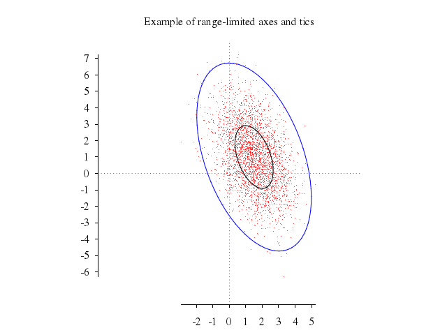
## axis ticmarks
[Original Demo](http://gnuplot.sourceforge.net/demo_4.6/tics.html)
### 1
```ruby
# # demo for tics settings
#
# set xlabel "x"
# set ylabel "y"
# set mxtics
#
# set title "Default tics settings"
# set xrange [-15:15]
# set yrange [-0.25:1]
# plot sin(sqrt(x**2))/sqrt(x**2) notitle
Numo.gnuplot do
set xlabel:"x"
set ylabel:"y"
set :mxtics
set title:"Default tics settings"
set xrange:-15..15
set yrange:-0.25..1
plot "sin(sqrt(x**2))/sqrt(x**2)", :notitle
end
```
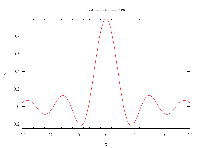
### 2
```ruby
# set title "Different modification of tics settings"
# set tics scale 3,2 rotate by 45
# set xtics out offset 0,-1.0
# replot
Numo.gnuplot do
set title:"Different modification of tics settings"
set :tics, :scale, [3,2], rotate_by:45
set :xtics, :out, offset:[0,-1.0]
replot
end
```
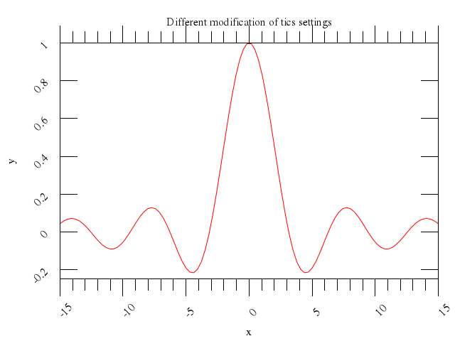
### 3
```ruby
# set xtics textcolor rgb "red" norotate
# set ytics rotate by 90 offset 2,0
# replot
Numo.gnuplot do
set :xtics, :textcolor, rgb:"red", norotate:true
set :ytics, :rotate, by:90, offset:[2,0]
replot
end
```
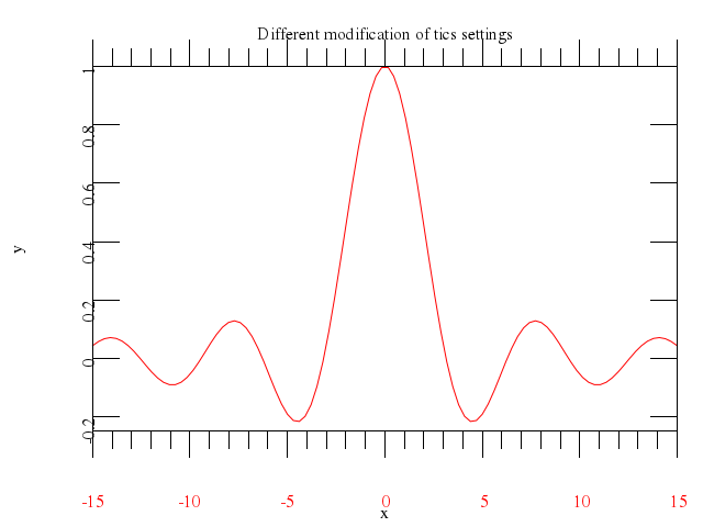
### 4
```ruby
# set title "Modification of tics settings (pm3d map with colorbar)"
# set pm3d map
# set border 4095
# set samples 25
# set isosamples 20
# set palette color positive
# set samples 50; set isosamples 50
# set tics norotate nooffset
# set cbtics in scale 4
# set xrange [-15:15]
# set yrange [-15:15]
# set zrange [-0.25:1]
# splot sin(sqrt(x**2+y**2))/sqrt(x**2+y**2) notitle
Numo.gnuplot do
set title:"Modification of tics settings (pm3d map with colorbar)"
set :pm3d, :map
set border:4095
set samples:25
set isosamples:20
set :palette, color:"positive"
set samples:50; set isosamples:50
set :tics, :norotate, :nooffset
set :cbtics, :in, scale:4
set xrange:-15..15
set yrange:-15..15
set zrange:-0.25..1
splot "sin(sqrt(x**2+y**2))/sqrt(x**2+y**2)", :notitle
end
```
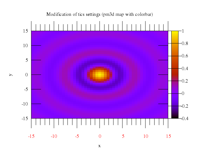
## rectangles
[Original Demo](http://gnuplot.sourceforge.net/demo_4.6/rectangle.html)
### 1
```ruby
# # demo for the use of "set object rectangle"
# #
# # Ethan A Merritt - 2006
#
# if ((GPVAL_VERSION == 4.3 || GPVAL_VERSION == 4.2) \
# && (!strstrt(GPVAL_COMPILE_OPTIONS,"+OBJECTS"))) \
# print ">>> Skipping demo <<<\n" ; \
# print "This copy of gnuplot was built without support for placing rectangles\n" ; \
# exit ;
#
# set style line 1 bgnd
# set style line 2 lt rgb "cyan"
#
# set object 1 rect from 0,0 to 1,4 fc lt 2
# set object 2 rect from -1,1 to 0,5 fc rgb "gold"
# set object 5 rect from 0, -3 to 2, -2 fc ls 2 fs pattern 1 bo -1
#
# set style fill pattern 2 bo 1
#
# #
# # Illustrate putting a different color under the key box
# #
# set key nobox
# set object 7 rect from graph 0.65,graph 0.85 to graph 0.99, graph 0.99 fc ls 1
#
# #
# # Illustrate using character widths to put a box around a label
# #
# LABEL = "Label in a box"
# set obj 10 rect at -3,-4 size char strlen(LABEL), char 1
# set obj 10 fillstyle empty border -1 front
# set label 10 LABEL at -3,-4 front center
#
# set obj 9 rect from -4, -4 to -4, -3 fc lt -1
#
# set obj 20 rect from graph 0, graph 0 to graph 1, graph 1 fs solid 0.15 fc rgb "#FFD700" behind
#
# plot [-5:5] x, -3+sin(x*5)/x lt 3 lw 3
Numo.gnuplot do
set :style, :line, 1, :bgnd
set :style, :line, 2, lt_rgb:"cyan"
set :object, 1, "rect", from:[0,0], to:[1,4], fc:true, lt:2
set :object, 2, "rect", from:[-1,1], to:[0,5], fc_rgb:"gold"
set :object, 5, "rect", from:[0,-3], to:[2,-2], fc:true, ls:2, fs:true, pattern:1, bo:-1
set :style, :fill, pattern:2, bo:1
set :key, :nobox
set :object, 7, "rect", from:"graph 0.65,graph 0.85", to:"graph 0.99, graph 0.99", fc:true, ls:1
run "LABEL = \"Label in a box\""
set :obj, 10, "rect", at:[-3,-4], size:"char strlen(LABEL), char 1"
set :obj, 10, :fillstyle, :empty, border:-1, front:true
set :label, 10, :'LABEL', at:[-3,-4], front:true, center:true
set :obj, 9, "rect", from:[-4,-4], to:[-4,-3], fc:true, lt:-1
set :obj, 20, "rect", from:"graph 0, graph 0", to:"graph 1, graph 1", fs_solid:0.15, fc_rgb:"#FFD700", behind:true
plot -5..5,
"x",
["-3+sin(x*5)/x", lt:3, lw:3]
end
```
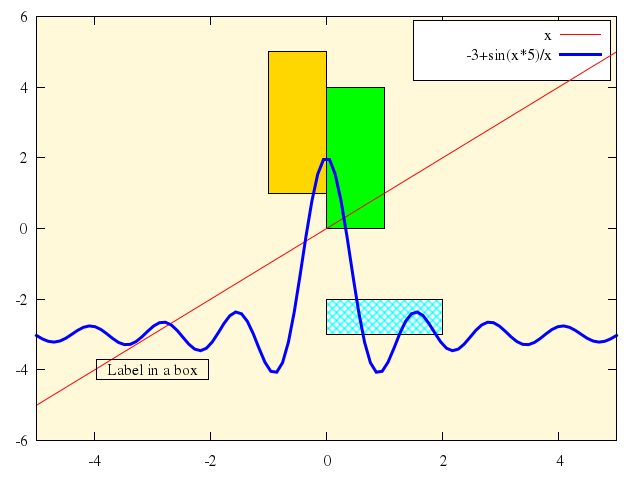
### 2
```ruby
# reset
#
# #
# # Requires data file "using.dat" from this directory,
# # so change current working directory to this directory before running.
# #
#
# set xrange [1:8]
# set title "Convex November 1-7 1989"
# set key below
# set label "(Weekend)" at 5,25 center
#
# set style rect fc lt -1 fs solid 0.15 noborder
#
# set obj rect from 1, graph 0 to 2, graph 1
# set obj rect from 3, graph 0 to 4, graph 1
# set obj rect from 5, graph 0 to 6, graph 1
# set obj rect from 7, graph 0 to 8, graph 1
#
# plot 'using.dat' using 3:4 title "Logged in" with impulses,\
# 'using.dat' using 3:5 t "Load average" with points,\
# 'using.dat' using 3:6 t "%CPU used" with lines
Numo.gnuplot do
reset
set xrange:1..8
set title:"Convex November 1-7 1989"
set :key, "below"
set label:"(Weekend)", at:[5,25], center:true
set :style, "rect", :fc, lt:-1, fs_solid:0.15, noborder:true
set :obj, "rect", from:"1, graph 0", to:"2, graph 1"
set :obj, "rect", from:"3, graph 0", to:"4, graph 1"
set :obj, "rect", from:"5, graph 0", to:"6, graph 1"
set :obj, "rect", from:"7, graph 0", to:"8, graph 1"
plot ["'using.dat'", using:[3,4], title:"Logged in", with:"impulses"],
["'using.dat'", using:[3,5], t:"Load average", with:"points"],
["'using.dat'", using:[3,6], t:"%CPU used", with:"lines"]
end
```
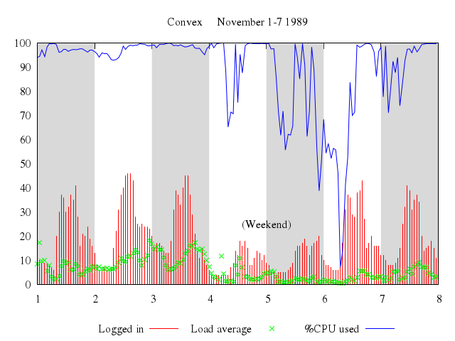
## line styles
[Original Demo](http://gnuplot.sourceforge.net/demo_4.6/dashcolor.html)
### 1
```ruby
# # Demonstrate explicit choice of both dot/dash pattern (linetype) and color (linecolor).
# #
# set termoption dash
#
# reset
# set xrange [-0.5:3.5]
# set yrange [-1:1.4]
# set bmargin 7
# unset ytics
# unset xtics
# #
# set title "Independent colors and dot/dash styles"
# unset colorbox
# #
# # define line styles using explicit rgbcolor names
# #
# set style line 1 lt 2 lc rgb "red" lw 3
# set style line 2 lt 2 lc rgb "orange" lw 2
# set style line 3 lt 2 lc rgb "yellow" lw 3
# set style line 4 lt 2 lc rgb "green" lw 2
# #
# set label 1 'set style line 1 lt 2 lc rgb "red" lw 3' at -0.4, -0.25 tc rgb "red"
# set label 2 'set style line 2 lt 2 lc rgb "orange" lw 2' at -0.4, -0.35 tc rgb "orange"
# set label 3 'set style line 3 lt 2 lc rgb "yellow" lw 3' at -0.4, -0.45 tc rgb "yellow"
# set label 4 'set style line 4 lt 2 lc rgb "green" lw 2' at -0.4, -0.55 tc rgb "green"
# set label 5 'plot ... lt 1 lc 3 ' at -0.4, -0.65 tc lt 3
# set label 6 'plot ... lt 3 lc 3 ' at -0.4, -0.75 tc lt 3
# set label 7 'plot ... lt 5 lc 3 ' at -0.4, -0.85 tc lt 3
# #
# set xlabel "You will only see dashed lines if your current terminal setting permits it"
# #
# show style line
# #
# # draw some plots
# #
# plot cos(x) ls 1 title 'ls 1', \
# cos(x-.2) ls 2 title 'ls 2',\
# cos(x-.4) ls 3 title 'ls 3',\
# cos(x-.6) ls 4 title 'ls 4', \
# cos(x-.8) lt 1 lc 3 title 'lt 1 lc 3', \
# cos(x-1.) lt 3 lc 3 title 'lt 3 lc 3', \
# cos(x-1.2) lt 5 lc 3 title 'lt 5 lc 3'
Numo.gnuplot do
set :termoption, :dash
reset
set xrange:-0.5..3.5
set yrange:-1..1.4
set bmargin:7
unset :ytics
unset :xtics
set title:"Independent colors and dot/dash styles"
unset :colorbox
set :style, :line, 1, lt:2, lc_rgb:"red", lw:3
set :style, :line, 2, lt:2, lc_rgb:"orange", lw:2
set :style, :line, 3, lt:2, lc_rgb:"yellow", lw:3
set :style, :line, 4, lt:2, lc_rgb:"green", lw:2
set :label, 1, 'set style line 1 lt 2 lc rgb "red" lw 3', at:[-0.4,-0.25], tc_rgb:"red"
set :label, 2, 'set style line 2 lt 2 lc rgb "orange" lw 2', at:[-0.4,-0.35], tc_rgb:"orange"
set :label, 3, 'set style line 3 lt 2 lc rgb "yellow" lw 3', at:[-0.4,-0.45], tc_rgb:"yellow"
set :label, 4, 'set style line 4 lt 2 lc rgb "green" lw 2', at:[-0.4,-0.55], tc_rgb:"green"
set :label, 5, 'plot ... lt 1 lc 3 ', at:[-0.4,-0.65], tc_lt:3
set :label, 6, 'plot ... lt 3 lc 3 ', at:[-0.4,-0.75], tc_lt:3
set :label, 7, 'plot ... lt 5 lc 3 ', at:[-0.4,-0.85], tc_lt:3
set xlabel:"You will only see dashed lines if your current terminal setting permits it"
show :style, :line
plot ["cos(x)", ls:1, title:'ls 1'],
["cos(x-.2)", ls:2, title:'ls 2'],
["cos(x-.4)", ls:3, title:'ls 3'],
["cos(x-.6)", ls:4, title:'ls 4'],
["cos(x-.8)", lt:1, lc:3, title:'lt 1 lc 3'],
["cos(x-1.)", lt:3, lc:3, title:'lt 3 lc 3'],
["cos(x-1.2)", lt:5, lc:3, title:'lt 5 lc 3']
end
```
### 2
```ruby
# unset for [i=1:8] label i
# set title "The pointinterval property is another way to create interrupted lines"
# set xlabel "This technique works best for equally spaced data points"
# set bmargin 6
# set offset .05, .05
# set xrange [-0.5:3.3]
# set style func linespoints
#
# plot cos(x) lt -1 pi -4 pt 6 title 'pi -4', \
# cos(x-.8) lt -1 pi -3 pt 7 ps 0.2 title 'pi -3 pt 7 ps 0.2', \
# cos(x-.2) lt -1 pi -6 pt 7 title 'pi -6',\
# cos(x-.4) lt -1 pi -3 pt 4 title 'pi -3',\
# cos(x-.6) lt -1 pi -5 pt 5 title 'pi -5', \
# cos(x-1.) with line lt -1 notitle, \
# cos(x+.2) with line lt -1 lw 2 title 'lw 2'
Numo.gnuplot do
unset "for [i=1:8] label i"
set title:"The pointinterval property is another way to create interrupted lines"
set xlabel:"This technique works best for equally spaced data points"
set bmargin:6
set offset:[0.05,0.05]
set xrange:-0.5..3.3
set :style, :func, :linespoints
plot ["cos(x)", lt:-1, pi:-4, pt:6, title:'pi -4'],
["cos(x-.8)", lt:-1, pi:-3, pt:7, ps:0.2, title:'pi -3 pt 7 ps 0.2'],
["cos(x-.2)", lt:-1, pi:-6, pt:7, title:'pi -6'],
["cos(x-.4)", lt:-1, pi:-3, pt:4, title:'pi -3'],
["cos(x-.6)", lt:-1, pi:-5, pt:5, title:'pi -5'],
["cos(x-1.)", with:"line", lt:-1, notitle:true],
["cos(x+.2)", with:"line", lt:-1, lw:2, title:'lw 2']
end
```
## fill styles
[Original Demo](http://gnuplot.sourceforge.net/demo_4.6/fillstyle.html)
### 1
```ruby
# # E A Merritt 24-Sep-2002
# #
# # Demo for revised fillstyle code selected by
# # ./configure --enable-filledboxes --enable-relative-boxwidth
# #
# reset
#
# set samples 25
# unset xtics
# unset ytics
# set yrange [0:120]
#
# set title "A demonstration of boxes with default properties"
# plot [-10:10] 100/(1.0+x*x) title 'distribution' with boxes
Numo.gnuplot do
reset
set samples:25
unset :xtics
unset :ytics
set yrange:0..120
set title:"A demonstration of boxes with default properties"
plot -10..10,
"100/(1.0+x*x)", title:'distribution', with:"boxes"
end
```
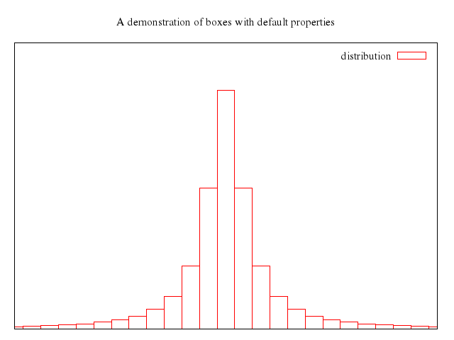
### 2
```ruby
# set title "A demonstration of boxes with style fill solid 1.0"
# set style fill solid 1.0
# replot
Numo.gnuplot do
set title:"A demonstration of boxes with style fill solid 1.0"
set :style, fill_solid:1.0
replot
end
```

### 3
```ruby
# set title "A demonstration of boxes with style fill solid border -1"
# set style fill solid border -1
# replot
Numo.gnuplot do
set title:"A demonstration of boxes with style fill solid border -1"
set :style, :fill_solid, border:-1
replot
end
```
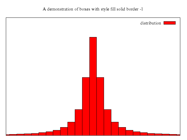
### 4
```ruby
# set title "Filled boxes of reduced width"
# set boxwidth 0.5
# replot
Numo.gnuplot do
set title:"Filled boxes of reduced width"
set boxwidth:0.5
replot
end
```
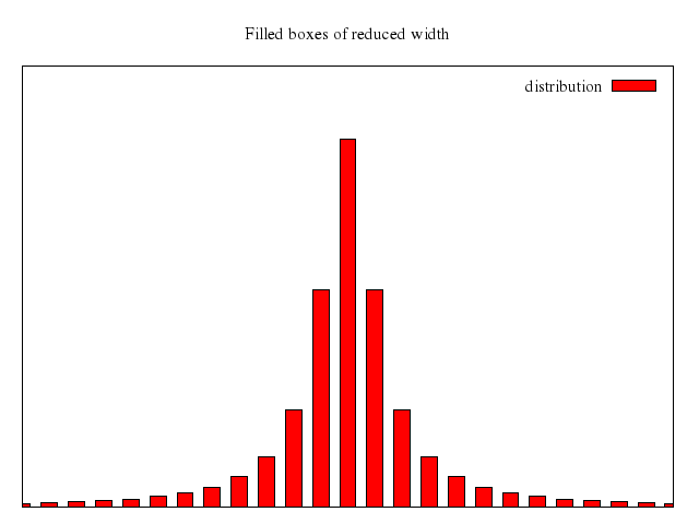
### 5
```ruby
# set title "Filled boxes at 50% fill density"
# set style fill solid 0.25 border
# replot
Numo.gnuplot do
set title:"Filled boxes at 50% fill density"
set :style, fill_solid:0.25, border:true
replot
end
```
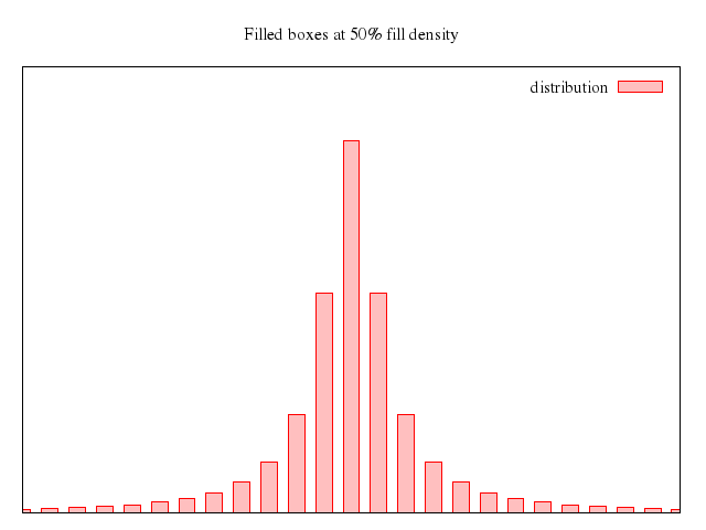
### 6
```ruby
# set title "A demonstration of boxes with style fill solid 0.25 noborder"
# set style fill solid 0.25 noborder
# replot
Numo.gnuplot do
set title:"A demonstration of boxes with style fill solid 0.25 noborder"
set :style, fill_solid:0.25, noborder:true
replot
end
```
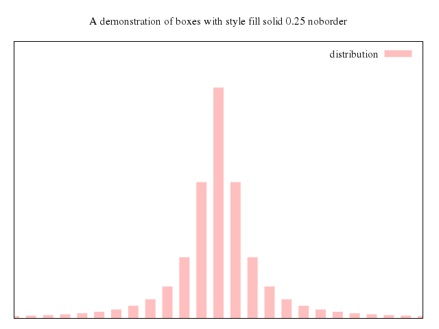
### 7
```ruby
# set title "A demonstration of boxes in mono with style fill pattern"
# set samples 11
# set boxwidth 0.5
# set style fill pattern border
# plot [-2.5:4.5] 100/(1.0+x*x) title 'pattern 0' with boxes lt -1, \
# 80/(1.0+x*x) title 'pattern 1' with boxes lt -1, \
# 40/(1.0+x*x) title 'pattern 2' with boxes lt -1, \
# 20/(1.0+x*x) title 'pattern 3' with boxes lt -1
Numo.gnuplot do
set title:"A demonstration of boxes in mono with style fill pattern"
set samples:11
set boxwidth:0.5
set :style, :fill, :pattern, :border
plot -2.5..4.5,
["100/(1.0+x*x)", title:'pattern 0', with:"boxes", lt:-1],
["80/(1.0+x*x)", title:'pattern 1', with:"boxes", lt:-1],
["40/(1.0+x*x)", title:'pattern 2', with:"boxes", lt:-1],
["20/(1.0+x*x)", title:'pattern 3', with:"boxes", lt:-1]
end
```
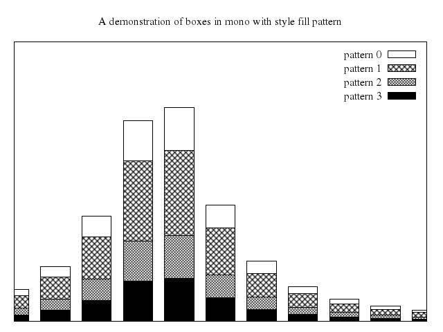
## arrow styles
[Original Demo](http://gnuplot.sourceforge.net/demo_4.6/arrowstyle.html)
### 1
```ruby
# set xrange [-1000:1000]
# set yrange [-178:86]
# set tics scale 0
#
# set style line 1 lt 1 lw 2
# set style line 2 lt 3 lw 2
#
# set style arrow 1 head filled size screen 0.025,30,45 ls 1
# set style arrow 2 head nofilled size screen 0.03,15 ls 2
# set style arrow 3 head filled size screen 0.03,15,45 ls 1
# set style arrow 4 head filled size screen 0.03,15 ls 2
# set style arrow 5 heads filled size screen 0.03,15,135 ls 1
# set style arrow 6 head empty size screen 0.03,15,135 ls 2
# set style arrow 7 nohead ls 1
# set style arrow 8 heads size screen 0.008,90 ls 2
#
# print ' We have defined the following arrowstyles:'
# show style arrow
#
# set arrow from -500,-100 to 500,-100 as 1
# set arrow from -500,-110 to 500,-110 as 2
# set arrow from -500,-120 to 500,-120 as 3
# set arrow from -500,-130 to 500,-130 as 4
# set arrow from -500,-140 to 500,-140 as 5
# set arrow from -500,-150 to 500,-150 as 6
# set arrow from -500,-160 to 500,-160 as 7
# set arrow from -500,-170 to 500,-170 as 8
#
# set label 'arrowstyle 1:' at -520,-100 right
# set label 'arrowstyle 2:' at -520,-110 right
# set label 'arrowstyle 3:' at -520,-120 right
# set label 'arrowstyle 4:' at -520,-130 right
# set label 'arrowstyle 5:' at -520,-140 right
# set label 'arrowstyle 6:' at -520,-150 right
# set label 'arrowstyle 7:' at -520,-160 right
# set label 'arrowstyle 8:' at -520,-170 right
#
# set title 'Top: plot with vectors arrowstyle 1, Bottom: explicit arrows'
# plot \
# 'arrowstyle.dat' using 1:2:(0):3 notitle with vectors arrowstyle 1
Numo.gnuplot do
set xrange:-1000..1000
set yrange:-178..86
set :tics, :scale, 0
set :style, :line, 1, lt:1, lw:2
set :style, :line, 2, lt:3, lw:2
set :style, arrow:1, head:true, filled:true, size_screen:[0.025,30,45], ls:1
set :style, arrow:2, head:true, nofilled:true, size_screen:[0.03,15], ls:2
set :style, arrow:3, head:true, filled:true, size_screen:[0.03,15,45], ls:1
set :style, arrow:4, head:true, filled:true, size_screen:[0.03,15], ls:2
set :style, arrow:5, heads:true, filled:true, size_screen:[0.03,15,135], ls:1
set :style, arrow:6, head:true, empty:true, size_screen:[0.03,15,135], ls:2
set :style, arrow:7, nohead:true, ls:1
set :style, arrow:8, heads:true, size_screen:[0.008,90], ls:2
show :style, :arrow
set :arrow, from:[-500,-100], to:[500,-100], as:1
set :arrow, from:[-500,-110], to:[500,-110], as:2
set :arrow, from:[-500,-120], to:[500,-120], as:3
set :arrow, from:[-500,-130], to:[500,-130], as:4
set :arrow, from:[-500,-140], to:[500,-140], as:5
set :arrow, from:[-500,-150], to:[500,-150], as:6
set :arrow, from:[-500,-160], to:[500,-160], as:7
set :arrow, from:[-500,-170], to:[500,-170], as:8
set label:'arrowstyle 1:', at:[-520,-100], right:true
set label:'arrowstyle 2:', at:[-520,-110], right:true
set label:'arrowstyle 3:', at:[-520,-120], right:true
set label:'arrowstyle 4:', at:[-520,-130], right:true
set label:'arrowstyle 5:', at:[-520,-140], right:true
set label:'arrowstyle 6:', at:[-520,-150], right:true
set label:'arrowstyle 7:', at:[-520,-160], right:true
set label:'arrowstyle 8:', at:[-520,-170], right:true
set title:'Top: plot with vectors arrowstyle 1, Bottom: explicit arrows'
plot "'arrowstyle.dat'", using:'1:2:(0):3', notitle:true, with:"vectors", arrowstyle:1
end
```
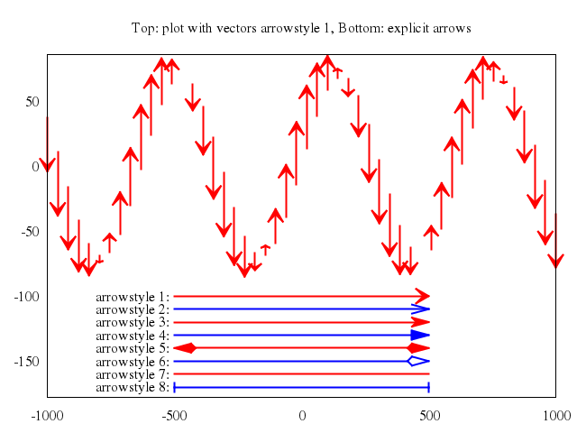
### 2
```ruby
# set title 'Top: plot with vectors arrowstyle 2, Bottom: explicit arrows'
# plot \
# 'arrowstyle.dat' using 1:2:(0):3 notitle with vectors arrowstyle 2
Numo.gnuplot do
set title:'Top: plot with vectors arrowstyle 2, Bottom: explicit arrows'
plot "'arrowstyle.dat'", using:'1:2:(0):3', notitle:true, with:"vectors", arrowstyle:2
end
```
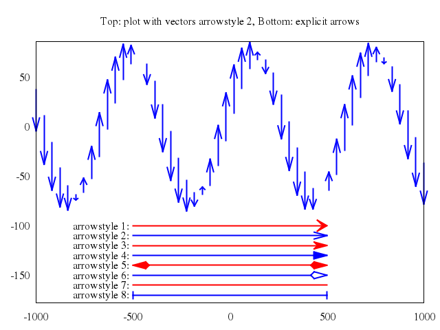
### 3
```ruby
# set title 'Top: plot with vectors arrowstyle 3, Bottom: explicit arrows'
# plot \
# 'arrowstyle.dat' using 1:2:(0):3 notitle with vectors arrowstyle 3
Numo.gnuplot do
set title:'Top: plot with vectors arrowstyle 3, Bottom: explicit arrows'
plot "'arrowstyle.dat'", using:'1:2:(0):3', notitle:true, with:"vectors", arrowstyle:3
end
```
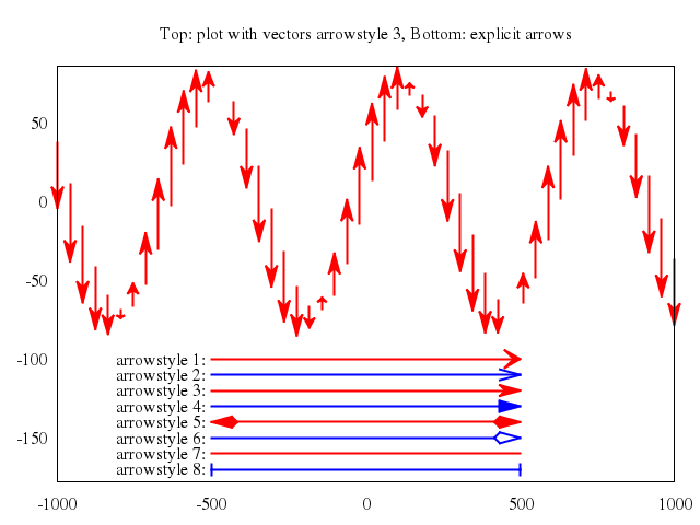
### 4
```ruby
# set title 'Top: plot with vectors arrowstyle 4, Bottom: explicit arrows'
# plot \
# 'arrowstyle.dat' using 1:2:(0):3 notitle with vectors arrowstyle 4
Numo.gnuplot do
set title:'Top: plot with vectors arrowstyle 4, Bottom: explicit arrows'
plot "'arrowstyle.dat'", using:'1:2:(0):3', notitle:true, with:"vectors", arrowstyle:4
end
```
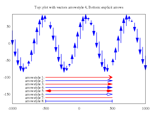
### 5
```ruby
# set title 'Top: plot with vectors arrowstyle 5, Bottom: explicit arrows'
# plot \
# 'arrowstyle.dat' using 1:2:(0):3 notitle with vectors arrowstyle 5
Numo.gnuplot do
set title:'Top: plot with vectors arrowstyle 5, Bottom: explicit arrows'
plot "'arrowstyle.dat'", using:'1:2:(0):3', notitle:true, with:"vectors", arrowstyle:5
end
```
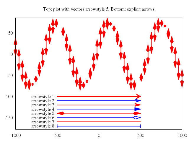
### 6
```ruby
# set title 'Top: plot with vectors arrowstyle 6, Bottom: explicit arrows'
# plot \
# 'arrowstyle.dat' using 1:2:(0):3 notitle with vectors arrowstyle 6
Numo.gnuplot do
set title:'Top: plot with vectors arrowstyle 6, Bottom: explicit arrows'
plot "'arrowstyle.dat'", using:'1:2:(0):3', notitle:true, with:"vectors", arrowstyle:6
end
```
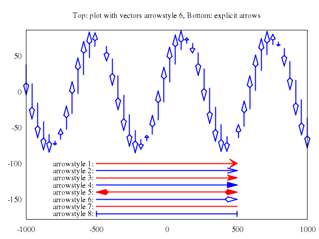
### 7
```ruby
# set title 'Top: plot with vectors arrowstyle 7, Bottom: explicit arrows'
# plot \
# 'arrowstyle.dat' using 1:2:(0):3 notitle with vectors arrowstyle 7
Numo.gnuplot do
set title:'Top: plot with vectors arrowstyle 7, Bottom: explicit arrows'
plot "'arrowstyle.dat'", using:'1:2:(0):3', notitle:true, with:"vectors", arrowstyle:7
end
```
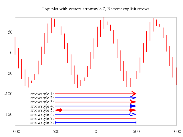
### 8
```ruby
# set title 'Top: plot with vectors arrowstyle 8, Bottom: explicit arrows'
# plot \
# 'arrowstyle.dat' using 1:2:(0):3 notitle with vectors arrowstyle 8
Numo.gnuplot do
set title:'Top: plot with vectors arrowstyle 8, Bottom: explicit arrows'
plot "'arrowstyle.dat'", using:'1:2:(0):3', notitle:true, with:"vectors", arrowstyle:8
end
```
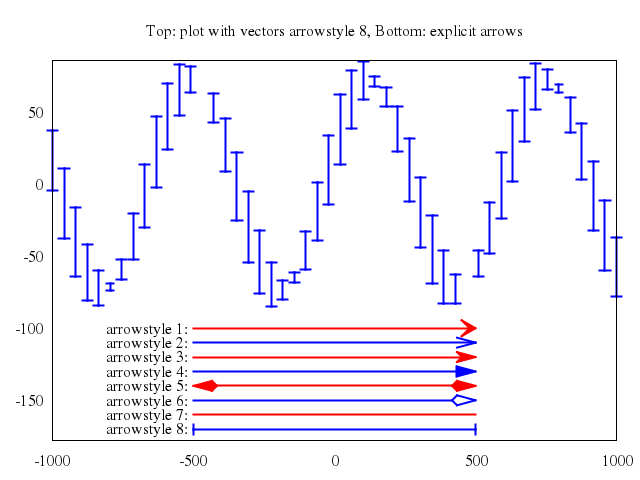
### 9
```ruby
# #reset
#
# #
# # Show plot with data style vectors
# #
# set title "Plot 'file' with vectors "
# set key box opaque
# set xrange [*:*]
# set yrange [*:10]
# set for [i=1:8] style arrow i lc i
# plot '1.dat' using 1:2:(+1):(+1) with vectors lt 4 filled title 'filled', \
# '2.dat' using 1:2:(+1):(+1) with vectors lt 1 heads title 'double-headed', \
# '2.dat' using ($1):(2-$2/3):(+1):(+2.5):(int($0)%8 + 1) with vectors as var ti 'arrowstyle variable'
Numo.gnuplot do
set title:"Plot 'file' with vectors "
set :key, :box, :opaque
set xrange:"[*:*]"
set yrange:"[*:10]"
set "for [i=1:8] style arrow i lc i"
plot ["'1.dat'", using:'1:2:(+1):(+1)', with:"vectors", lt:4, filled:true, title:'filled'],
["'2.dat'", using:'1:2:(+1):(+1)', with:"vectors", lt:1, heads:true, title:'double-headed'],
["'2.dat'", using:'($1):(2-$2/3):(+1):(+2.5):(int($0)%8 + 1)', with:"vectors", as:"var", ti:'arrowstyle variable']
end
```
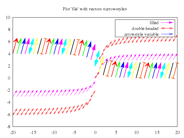
## transparency
[Original Demo](http://gnuplot.sourceforge.net/demo_4.6/transparent.html)
### 1
```ruby
# # Example of transparent fill areas
# # Ethan A Merritt - Aug 2006
# # NB:
# # Not all terminal types support transparency
# # Assumes UTF-8 support for plot titles
# #
# set style fill solid 1.0 noborder
# set style function filledcurves y1=0
# set clip two
#
# Gauss(x,mu,sigma) = 1./(sigma*sqrt(2*pi)) * exp( -(x-mu)**2 / (2*sigma**2) )
# d1(x) = Gauss(x, 0.5, 0.5)
# d2(x) = Gauss(x, 2., 1.)
# d3(x) = Gauss(x, -1., 2.)
#
# set xrange [-5:5]
# set yrange [0:1]
#
# unset colorbox
#
# set key title "Gaussian Distribution"
# set key top left Left reverse samplen 1
#
# #set obj 1 rect from graph 0,0 to graph 1,1
# #set obj 1 rect back fs solid 0.25 fc lt 4
#
# set title "Solid filled curves"
# plot d1(x) fs solid 1.0 lc rgb "forest-green" title "μ = 0.5 σ = 0.5", \
# d2(x) lc rgb "gold" title "μ = 2.0 σ = 1.0", \
# d3(x) lc rgb "red" title "μ = -1.0 σ = 2.0"
Numo.gnuplot do
set :style, fill_solid:1.0, noborder:true
set :style, function:'filledcurves y1=0'
set clip:"two"
run "Gauss(x,mu,sigma) = 1./(sigma*sqrt(2*pi)) * exp( -(x-mu)**2 / (2*sigma**2) )"
run "d1(x) = Gauss(x, 0.5, 0.5)"
run "d2(x) = Gauss(x, 2., 1.)"
run "d3(x) = Gauss(x, -1., 2.)"
set xrange:-5..5
set yrange:0..1
unset :colorbox
set :key, title:"Gaussian Distribution"
set :key, :top, :left, :Left, :reverse, samplen:1
set title:"Solid filled curves"
plot ["d1(x)", fs_solid:1.0, lc_rgb:"forest-green", title:"μ = 0.5 σ = 0.5"],
["d2(x)", lc_rgb:"gold", title:"μ = 2.0 σ = 1.0"],
["d3(x)", lc_rgb:"red", title:"μ = -1.0 σ = 2.0"]
end
```
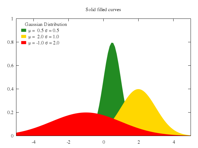
### 2
```ruby
# set style fill transparent solid 0.5 noborder
# set title "Transparent filled curves"
# replot
Numo.gnuplot do
set :style, fill:"transparent", solid:0.5, noborder:true
set title:"Transparent filled curves"
replot
end
```
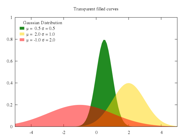
### 3
```ruby
# set style fill pattern 4 bo
# set title "Pattern-filled curves"
# replot
Numo.gnuplot do
set :style, :fill, pattern:4, bo:true
set title:"Pattern-filled curves"
replot
end
```
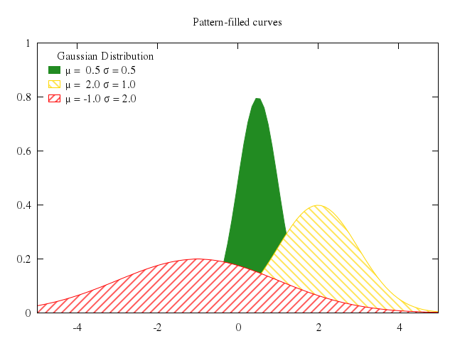
### 4
```ruby
# set style fill transparent pattern 4 bo
# set title "Transparent pattern-filled curves"
# replot
Numo.gnuplot do
set :style, fill:"transparent", pattern:4, bo:true
set title:"Transparent pattern-filled curves"
replot
end
```
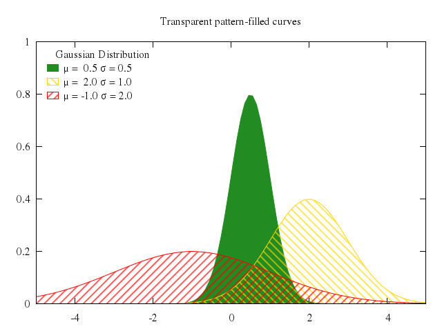
## transparent solids
[Original Demo](http://gnuplot.sourceforge.net/demo_4.6/transparent_solids.html)
### 1
```ruby
# set title "Interlocking Tori - PM3D surface with depth sorting and transparency"
#
# unset border
# unset key
# set object 1 rect from screen 0, 0, 0 to screen 1, 1, 0 behind
# set object 1 rect fc rgb "gray" fillstyle solid 1.0 border -1
# set view 64, 345, 1.24375, 0.995902
# set isosamples 50, 20
# unset xtics
# unset ytics
# unset ztics
# set parametric
# set dummy u,v
# set urange [ -pi : pi ]
# set vrange [ -pi : pi ]
#
# set pm3d depthorder hidden3d 2
# set palette rgbformulae 8, 9, 7
# set style line 2 linetype 2 linecolor rgb "#a0a0f0" linewidth 0.5
# set style fill transparent solid 0.30 border
#
# splot cos(u)+.5*cos(u)*cos(v),sin(u)+.5*sin(u)*cos(v),.5*sin(v) with pm3d, \
# 1+cos(u)+.5*cos(u)*cos(v),.5*sin(v),sin(u)+.5*sin(u)*cos(v) with pm3d
Numo.gnuplot do
set title:"Interlocking Tori - PM3D surface with depth sorting and transparency"
unset :border
unset :key
set :object, 1, "rect", from_screen:[0,0,0], to_screen:[1,1,0], behind:true
set :object, 1, "rect", fc_rgb:"gray", fillstyle_solid:1.0, border:-1
set view:[64,345,1.24375,0.995902]
set isosamples:[50,20]
unset :xtics
unset :ytics
unset :ztics
set :parametric
set dummy:"u,v"
set urange:"[-pi:pi]"
set vrange:"[-pi:pi]"
set :pm3d, "depthorder", hidden3d:2
set :palette, rgbformulae:[8,9,7]
set :style, :line, 2, linetype:2, linecolor_rgb:"#a0a0f0", linewidth:0.5
set :style, fill:"transparent", solid:0.30, border:true
splot "cos(u)+.5*cos(u)*cos(v)",
"sin(u)+.5*sin(u)*cos(v)",
[".5*sin(v)", with:"pm3d"],
"1+cos(u)+.5*cos(u)*cos(v)",
".5*sin(v)",
["sin(u)+.5*sin(u)*cos(v)", with:"pm3d"]
end
```
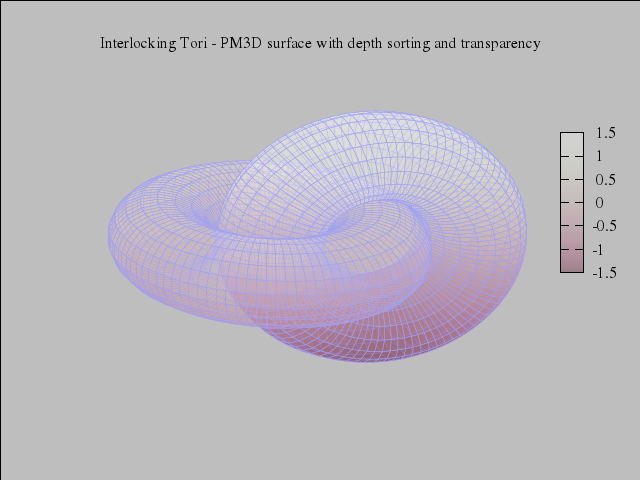
### 2
```ruby
# unset title
# set label 1 "Kuen's Surface" at screen 0.57, 0.9
# set label 1 font "frscript,20"
# set style line 3 linetype -1 linewidth 0.5
# set pm3d depthorder hidden3d 3
# set style fill transparent solid 0.65 border
# set palette
# set hidden3d
#
# set ticslevel 0
# unset xtics ; unset ytics ; unset ztics
# unset border ; unset colorbox ; unset key
# set lmargin at screen 0.1
# set bmargin at screen 0.1
# set rmargin at screen 0.9
# set tmargin at screen 0.9
#
# set parametric
# set dummy u,v
# set urange [-4.5:4.5]
# set vrange [0.05:pi-0.05]
# set isosamples 51,51
# set view 122, 357, 1.35, 1.08
#
# a = 1.0
#
# x(u,v) = 2.*a*(cos(u)+u*sin(u))*sin(v) / (1+u**2.*(sin(v))**2)
# y(u,v) = 2.*a*(sin(u)-u*cos(u))*sin(v) / (1+u**2.*(sin(v))**2)
# z(u,v) = a*log(tan(v/2.))+2.*cos(v)/(1+u**2.*(sin(v))**2)
#
# splot x(u,v), y(u,v), z(u,v) with pm3d
Numo.gnuplot do
unset :title
set :label, 1, "Kuen's Surface", at_screen:[0.57,0.9]
set :label, 1, font:"frscript,20"
set :style, :line, 3, linetype:-1, linewidth:0.5
set :pm3d, "depthorder", hidden3d:3
set :style, fill:"transparent", solid:0.65, border:true
set :palette
set :hidden3d
set ticslevel:0
unset :xtics; unset :ytics; unset :ztics
unset :border; unset :colorbox; unset :key
set :lmargin, :at, screen:0.1
set :bmargin, :at, screen:0.1
set :rmargin, :at, screen:0.9
set :tmargin, :at, screen:0.9
set :parametric
set dummy:"u,v"
set urange:-4.5..4.5
set vrange:"[0.05:pi-0.05]"
set isosamples:[51,51]
set view:[122,357,1.35,1.08]
run "a = 1.0"
run "x(u,v) = 2.*a*(cos(u)+u*sin(u))*sin(v) / (1+u**2.*(sin(v))**2)"
run "y(u,v) = 2.*a*(sin(u)-u*cos(u))*sin(v) / (1+u**2.*(sin(v))**2)"
run "z(u,v) = a*log(tan(v/2.))+2.*cos(v)/(1+u**2.*(sin(v))**2)"
splot "x(u,v)",
"y(u,v)",
["z(u,v)", with:"pm3d"]
end
```
