Extensible visualization using HadoopViz
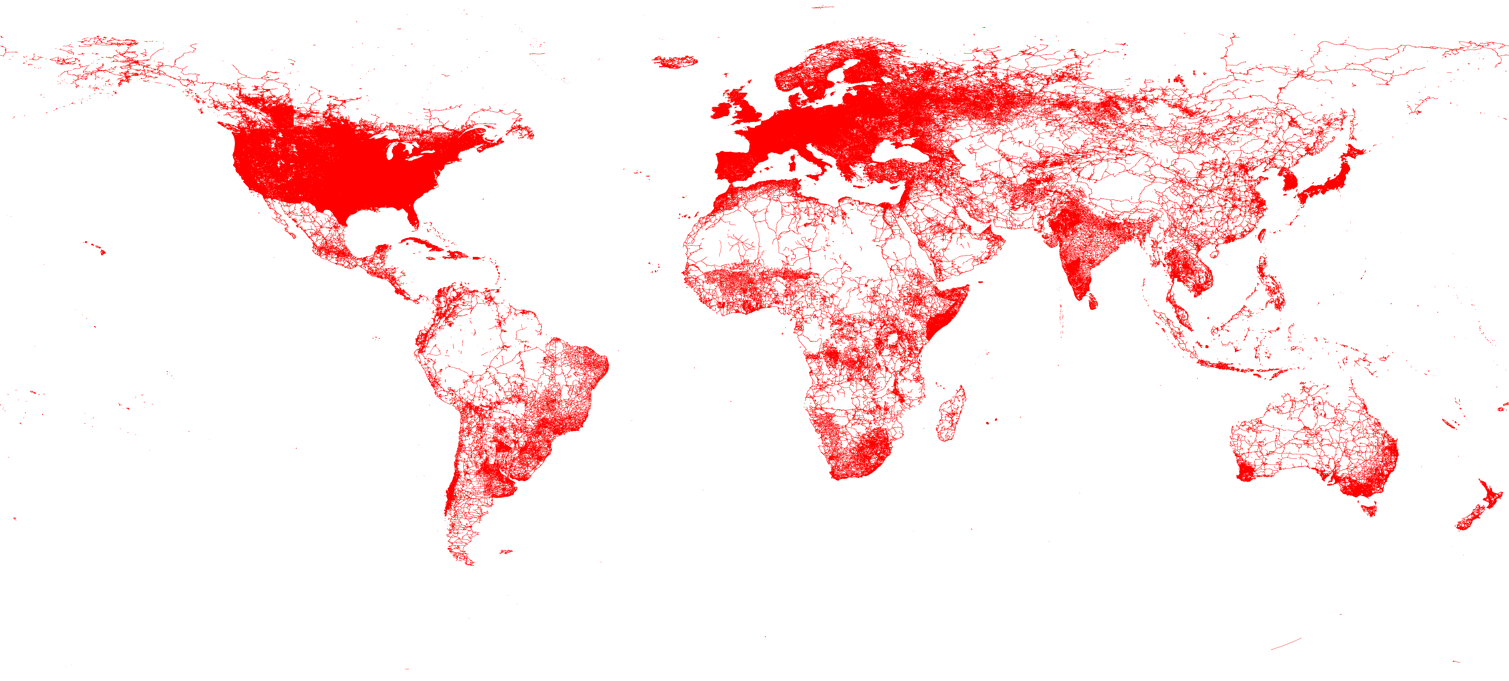
SpatialHadoop provides efficient tools for visualization of large files. This functionality is greatly useful when you have a very large file and you want to explore it by creating an image out of it. For example, the image shown below visualizes all road networks on the planet. This image is created from a dataset of 59 Million lines with a total size of 20.6GB. The dataset is extracted from OpenStreetMap and can be download for free on the datasets page.
SpatialHadoop contains an extensible interface for visualization which separates the visualization logic from the implementation of the visualization algorithm. The user can easily define a new type of visualization by extending the abstract class Plotter. The implementing class can be plugged into the visualization algorithms provided in SpatialHadoop to work as a MapReduce program to generate either a single-level image or multilevel image. In this tutorial, we first describe how the abstract interface looks like and how to use it to generate both types of images.
SpatialHadoop supports two types of images, namely, single level and multilevel images. A single level image is an image of a fixed resolution that can be viewed using any image viewer or embedded in a document such as a website or a report. The quality of the image is limited by the resolution of the image. The image shown above is an example of a single level image. A multilevel image is composed of many small image tiles generated for different regions at different zoom levels. This allows the user to zoom into the image or pan around to see more details about a specific area. This technique is already used in most web-based maps such as Google Maps (Satellite view), Bing Maps and OpenStreetMap. For example, this image shows a multilevel image of the road segments in Minnesota extracted from OpenStreetMap data.
Both image types are supported by SpatialHadoop through a common interface. We define a general visualization interface that can be implemented once and used to generate both single and multilevel images.
The visualization interface is defined in the abstract class Plotter. It contains five main methods that define the visualization logic.
-
smooth: This optional function can be defined to fuse nearby together to improve the generate image. For example, when visualizing a road network, this method can be used to merge intersecting road segments. -
createCanvas: This method initializes an in-memory object which will act as a canvas on which records will be plotted. For example, it can be an in-memory image on which records are drawn or a two-dimensional histogram on which data are aggregated -
plot: This method takes a canvas previously created using createCanvas and a shape, then it plots (i.e., draws) this shape on the canvas. -
merge: This method takes two canvases and merges them together into one canvas. This is used to merge partial images into one final image before it is written to the output is a single image. -
writeImage: This method is called once at the end to write the final image to the output in a standard image format.
Let us say you have a new type of data that you want to visualize in a customized way. First, you need to create a new rasterizer as a class that implements the Rasterizer interface. Once you implement this class, you need to use either the SingleLevelPlot or MultilevelPlot classes to generate a single level or multilevel images, respectively. Both of them contain a method that accepts a class that extends the Rasterizer and use it to visualize an input data using MapReduce.
Case Study I: Geometric Plot
The geometric plot operation implements a simple rasterizer that draws the geometry of shapes on a normal image. For example, it generates a scatter plot out of a point dataset or draws a set of polygons on an image. The rasterizer of this operation is implemented as follows:
-
smooth: No smooth function is implemented for this operation -
createCanvas: Initializes an in-memory image of the given resolution with a transparent background -
plot: Draws the geometry of a shape on the in-memory image. For example, a point is represented as a pixel while a polygon is drawn using the Graphics#drawPolygon method. -
merge: Plots one image on top of the other image. The transparent background initialized for each image allows the image on top to reveal the image beneath it. -
writeImage: The image is written to the output in a standard PNG format using the ImageIO class.
Case Study II: Heat Map Plot
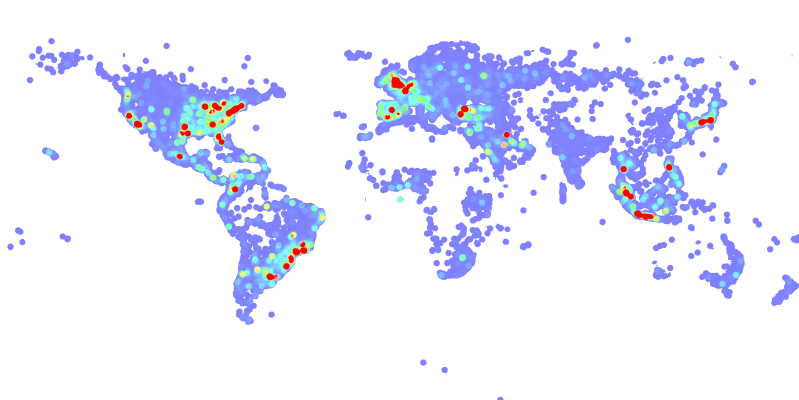
This visualization technique is applied to an input file that contains points. It gives a color to each pixel in the generated image according to the density of points around this pixel. An example of the heat map of tweets in one day is shown below (click the image to enlarge).
In this image, areas with low density of tweets are colored in blue while areas of higher densities are colored in red. The functions for this operation are implemented as follows:
-
smooth: No smooth function is implemented for this method -
createCanvas: Initializes a frequency map as a two-dimensional array of integers where each entry corresponds to a pixel in the image and holds the total number of points around it -
plot: Takes a point and updates the frequency map by incrementing all points around its location. -
merge: Merges two frequency map by adding up corresponding entries in both frequency maps. -
writeImage: This method first converts the frequency map into an image by mapping each entry to a pixel and color it with the corresponding color according to its value. After that, it writes the resulted image as a PNG image using the ImageIO class.