---

PathSim - A System Simulation Framework

Overview

PathSim is a flexible block-based time-domain system simulation framework in Python with automatic differentiation capabilities and an event handling mechanism! It provides a variety of classes that enable modeling and simulating complex interconnected dynamical systems through Python scripting.

All of that with minimal dependencies, only numpy, scipy and matplotlib (and dill if you want to use serialization)!

Key Features:

• Dynamic system modification at simulation runtime, i.e. triggered through events
• Automatic block- and system-level linearization at runtime
• Wide range of numerical integrators (implicit, explicit, high order, adaptive), able to handle stiff systems
• Modular and hierarchical modeling with (nested) subsystems
• Event handling system to detect and resolve discrete events (zero-crossing detection)
• Automatic differentiation for end-to-end differentiable simulations
• Extensibility by subclassing the base Block class and implementing just a handful of methods

For the full documentation, tutorials and API-reference visit Read the Docs!

The source code can be found in the GitHub repository and is fully open source under MIT license. Consider starring PathSim to support its development.

Installation

The latest release version of PathSim is available on PyPi and installable via pip:

pip install pathsim

Example - Harmonic Oscillator

There are lots of examples of dynamical system simulations in the GitHub repository that showcase PathSim's capabilities.

But first, lets have a look at how we can simulate the harmonic oscillator (a spring mass damper 2nd order system) using PathSim. The system and its corresponding equivalent block diagram are shown in the figure below:

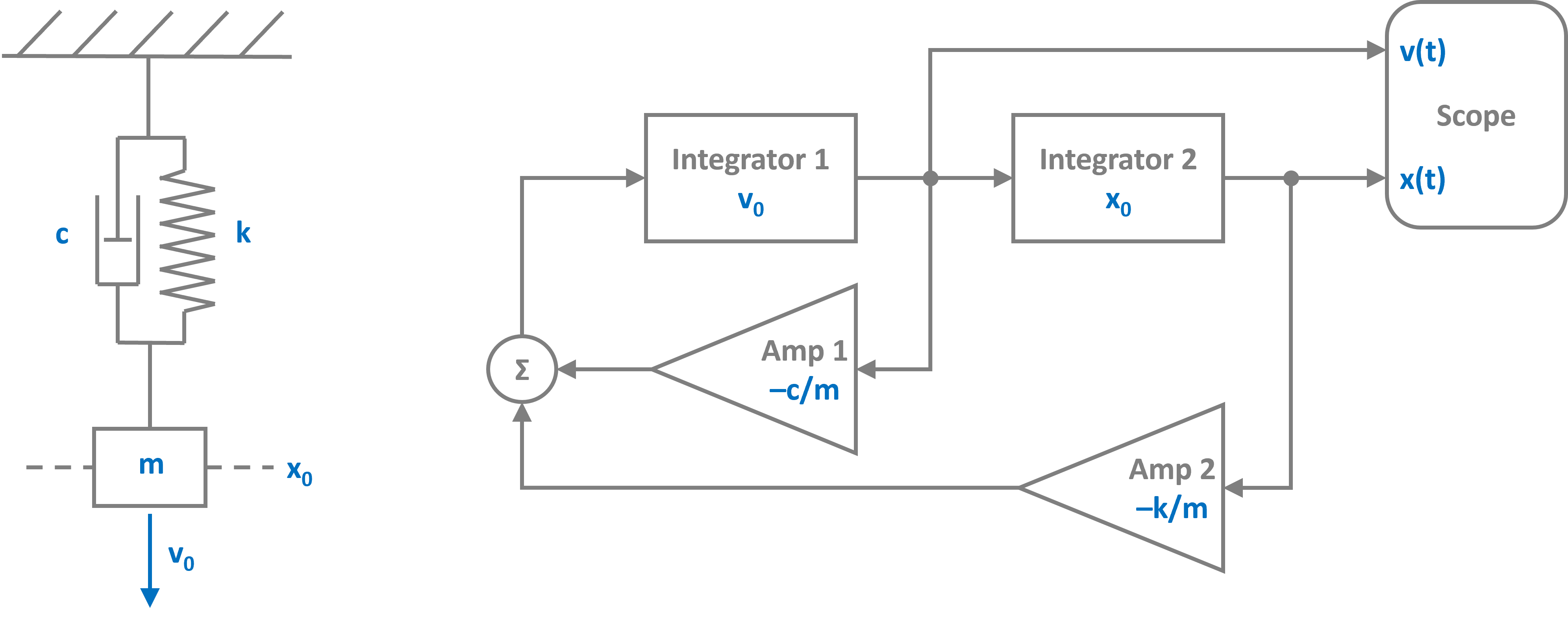
The equation of motion that defines the harmonic oscillator it is give by

$$ \ddot{x} + \frac{c}{m} \dot{x} + \frac{k}{m} x = 0 $$

where $c$ is the damping, $k$ the spring constant and $m$ the mass together with the initial conditions $x_0$ and $v_0$ for position and velocity.

The topology of the block diagram above can be directly defined as blocks and connections in the PathSim framework. First we initialize the blocks needed to represent the dynamical systems with their respective arguments such as initial conditions and gain values, then the blocks are connected using Connection objects, forming two feedback loops.

The Simulation instance manages the blocks and connections and advances the system in time with the timestep (dt). The log flag for logging the simulation progress is also set. Finally, we run the simulation for some number of seconds and plot the results using the plot() method of the scope block.

from pathsim import Simulation, Connection

#import the blocks we need for the harmonic oscillator
from pathsim.blocks import Integrator, Amplifier, Adder, Scope

#initial position and velocity
x0, v0 = 2, 5

#parameters (mass, damping, spring constant)
m, c, k = 0.8, 0.2, 1.5

#define the blocks 
I1 = Integrator(v0)   # integrator for velocity
I2 = Integrator(x0)   # integrator for position
A1 = Amplifier(-c/m)
A2 = Amplifier(-k/m)
P1 = Adder()
Sc = Scope(labels=["v(t)", "x(t)"])

blocks = [I1, I2, A1, A2, P1, Sc]

#define the connections between the blocks
connections = [
    Connection(I1, I2, A1, Sc),   # one to many connection
    Connection(I2, A2, Sc[1]),
    Connection(A1, P1),           # default connection to port 0
    Connection(A2, P1[1]),        # specific connection to port 1
    Connection(P1, I1)
    ]

#create a simulation instance from the blocks and connections
Sim = Simulation(blocks, connections, dt=0.05)

#run the simulation for 30 seconds
Sim.run(duration=30.0)

#plot the results directly from the scope
Sc.plot()

#read the results from the scope for further processing
time, data = Sc.read()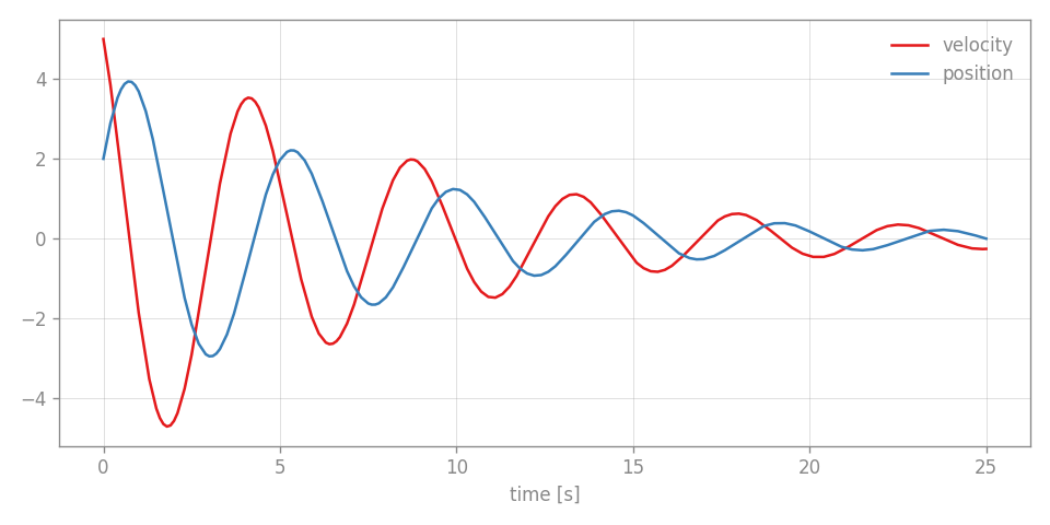

Stiff Systems

PathSim implements a large variety of implicit integrators such as diagonally implicit runge-kutta (DIRK2, ESDIRK43, etc.) and multistep (BDF2, GEAR52A, etc.) methods. This enables the simulation of very stiff systems where the timestep is limited by stability and not accuracy of the method.

A common example for a stiff system is the Van der Pol oscillator where the parameter $\mu$ "controls" the severity of the stiffness. It is defined by the following second order ODE:

$$ \ddot{x} + \mu (1 - x^2) \dot{x} + x = 0 $$

The Van der Pol ODE can be translated into a block diagram like the one below, where the two states are handled by two distinct integrators.

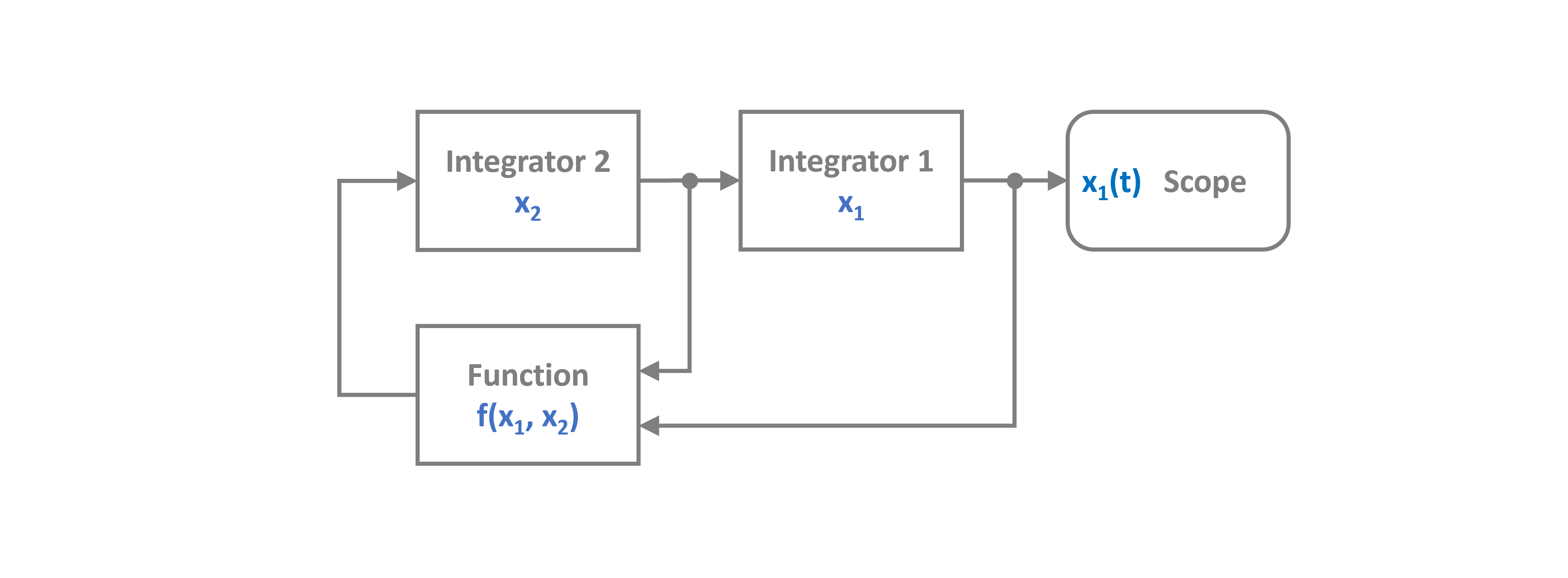
Lets translate it to PathSim using two Integrator blocks and a Function block. The parameter is set to $\mu = 1000$ which means severe stiffness.

from pathsim import Simulation, Connection
from pathsim.blocks import Integrator, Scope, Function

#implicit adaptive timestep solver 
from pathsim.solvers import ESDIRK54

#initial conditions
x1, x2 = 2, 0

#van der Pol parameter (1000 is very stiff)
mu = 1000

#blocks that define the system
Sc = Scope(labels=["$x_1(t)$"])
I1 = Integrator(x1)
I2 = Integrator(x2)
Fn = Function(lambda x1, x2: mu*(1 - x1**2)*x2 - x1)

blocks = [I1, I2, Fn, Sc]

#the connections between the blocks
connections = [
    Connection(I2, I1, Fn[1]), 
    Connection(I1, Fn, Sc), 
    Connection(Fn, I2)
    ]

#initialize simulation with the blocks, connections, timestep and logging enabled
Sim = Simulation(
    blocks, 
    connections, 
    dt=0.05, 
    Solver=ESDIRK54, 
    tolerance_lte_abs=1e-5, 
    tolerance_lte_rel=1e-3
    )

#run simulation for some number of seconds
Sim.run(3*mu)

#plot the results directly (steps highlighted)
Sc.plot(".-")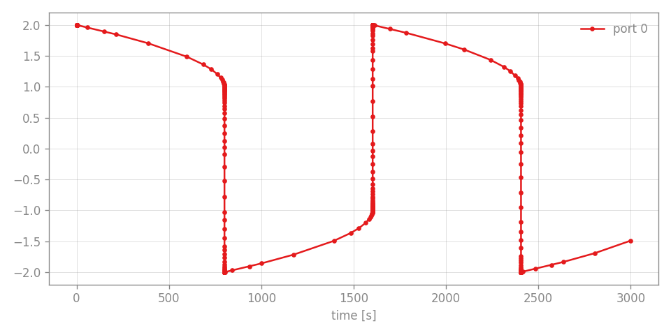

Differentiable Simulation

PathSim also includes a fully fledged automatic differentiation framework based on a dual number system with overloaded operators and numpy ufunc integration. This makes the system simulation fully differentiable end-to-end with respect to a predefined set of parameters. Works with all integrators, adaptive, fixed, implicit, explicit.

To demonstrate this lets consider the following linear feedback system and perform a sensitivity analysis on it with respect to some system parameters.

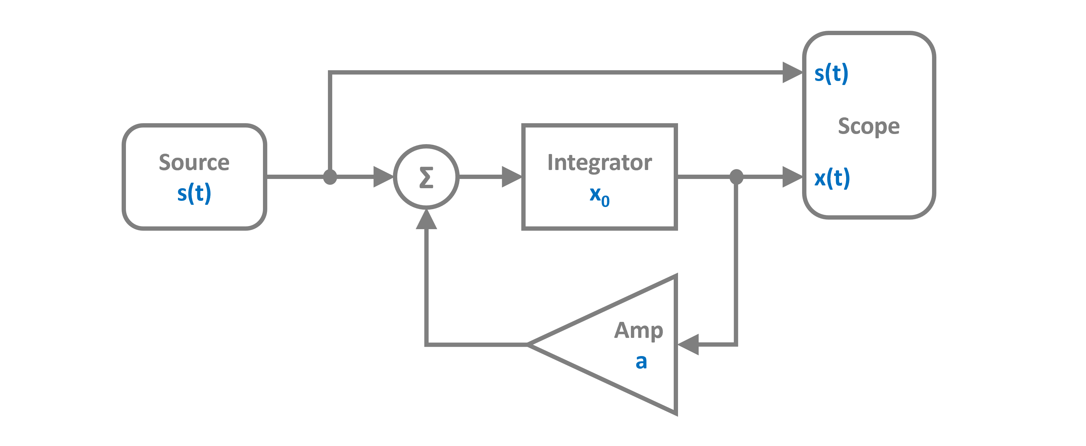
The source term is a scaled unit step function (scaled by $b$). In this example, the parameters for the sensitivity analysis are the feedback term $a$, the initial condition $x_0$ and the amplitude of the source term $b$.

from pathsim import Simulation, Connection
from pathsim.blocks import Source, Integrator, Amplifier, Adder, Scope

#AD module
from pathsim.optim import Value, der

#values for derivative propagation / parameters for sensitivity analysis
a  = Value(-1)
b  = Value(1)
x0 = Value(2)

#simulation timestep
dt = 0.01

#step function
tau = 3
def s(t):
    return b*int(t>tau)

#blocks that define the system
Src = Source(s)
Int = Integrator(x0)
Amp = Amplifier(a)
Add = Adder()
Sco = Scope(labels=["step", "response"])

blocks = [Src, Int, Amp, Add, Sco]

#the connections between the blocks
connections = [
    Connection(Src, Add[0], Sco[0]),
    Connection(Amp, Add[1]),
    Connection(Add, Int),
    Connection(Int, Amp, Sco[1])
    ]

#initialize simulation with the blocks, connections, timestep
Sim = Simulation(blocks, connections, dt=dt)
    
#run the simulation for some time
Sim.run(4*tau)

Sco.plot()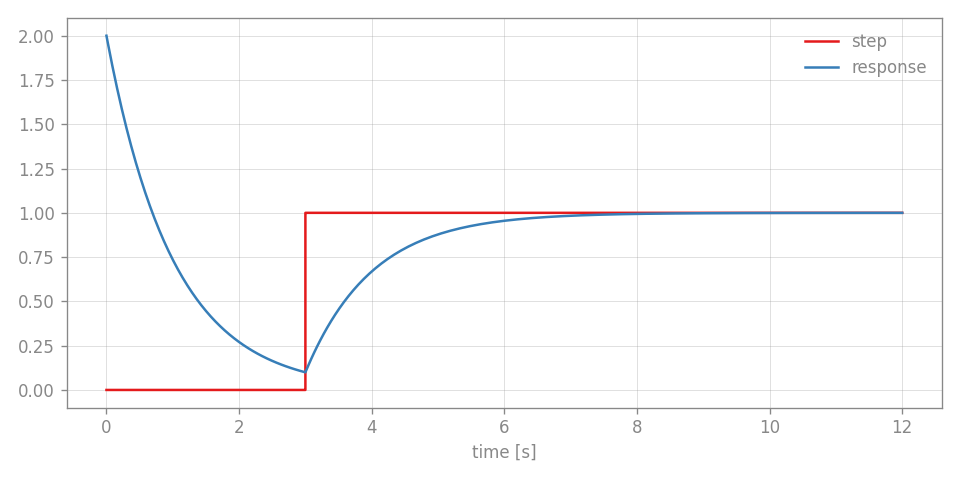

Now the recorded time series data is of type Value and we can evaluate the automatically computed partial derivatives at each timestep. For example the response, differentiated with respect to the linear feedback parameter $\partial x(t) / \partial a$ can be extracted from the data like this der(data, a).

import matplotlib.pyplot as plt

#read data from the scope
time, [step, data] = Sco.read()

fig, ax = plt.subplots(nrows=1, tight_layout=True, figsize=(8, 4), dpi=120)

#evaluate and plot partial derivatives
ax.plot(time, der(data, a), label=r"$\partial x / \partial a$")
ax.plot(time, der(data, x0), label=r"$\partial x / \partial x_0$")
ax.plot(time, der(data, b), label=r"$\partial x / \partial b$")

ax.set_xlabel("time [s]")
ax.grid(True)
ax.legend(fancybox=False)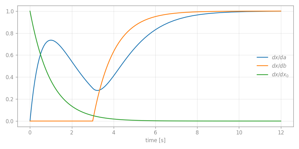

Event Detection

PathSim has an event handling system that monitors the simulation state and can find and locate discrete events by evaluating an event function and trigger callbacks or state transformations. Multiple event types are supported such as ZeroCrossing or Schedule.

This enables the simulation of hybrid continuous time systems with discrete events.

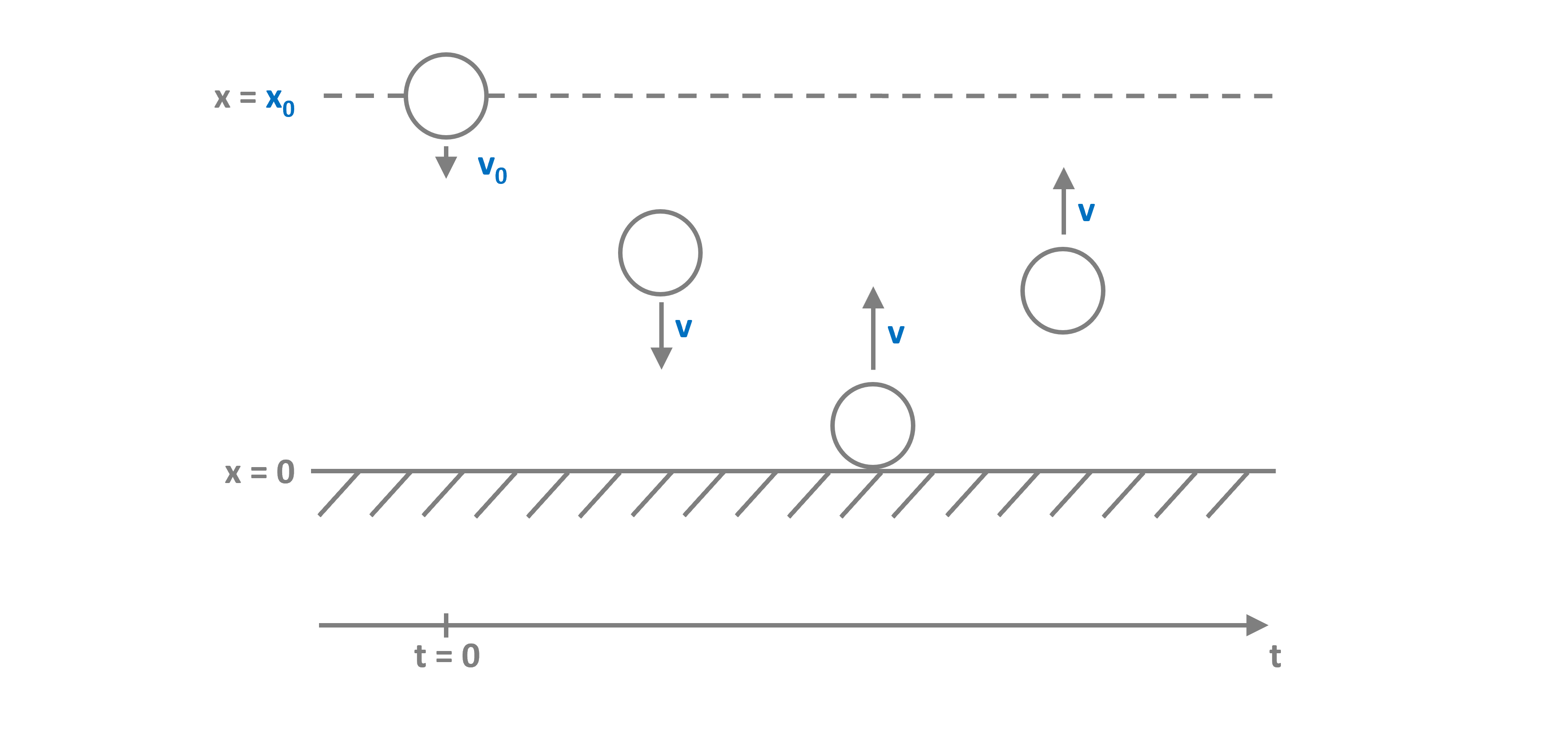
Probably the most popular example for this is the bouncing ball (see figure above) where discrete events occur whenever the ball touches the floor. The event in this case is a zero-crossing.

The dynamics of this system can be translated into a block diagramm in the following way:

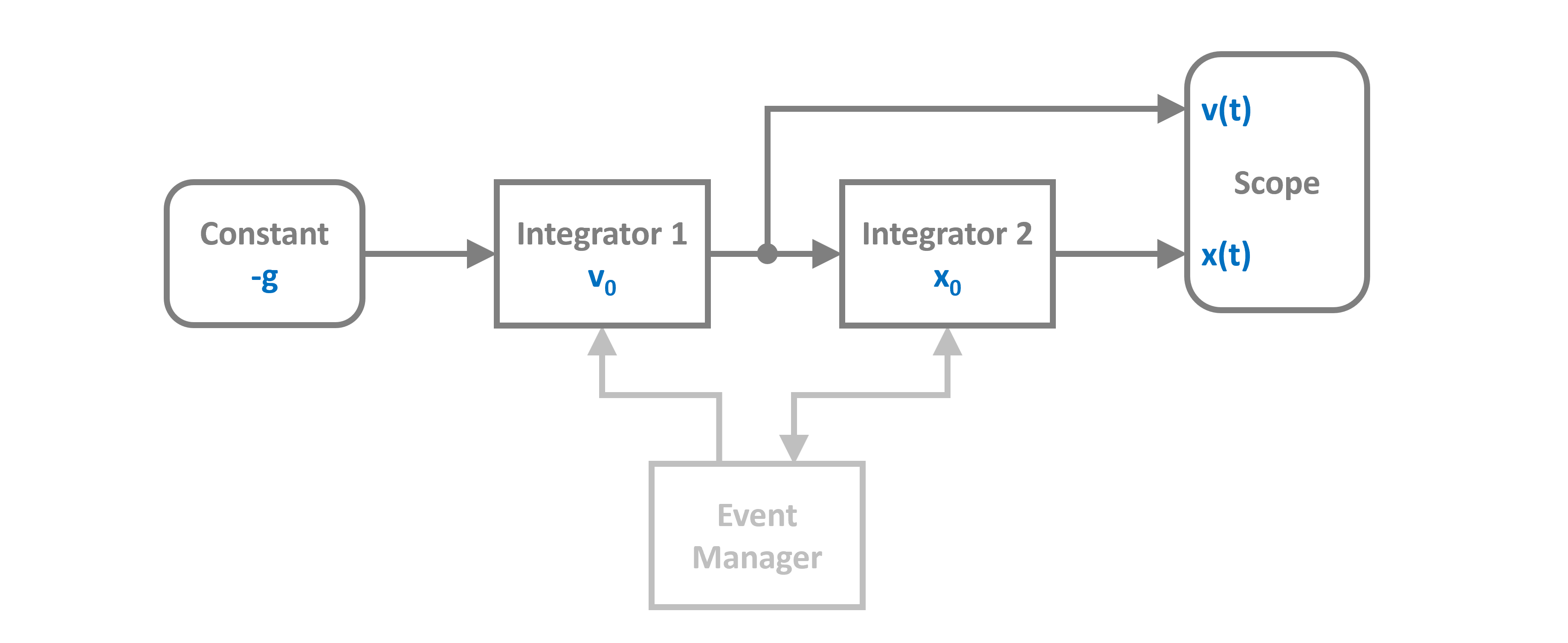
And built and simulated with PathSim like this:

from pathsim import Simulation, Connection
from pathsim.blocks import Integrator, Constant, Scope
from pathsim.solvers import RKBS32

#event library
from pathsim.events import ZeroCrossing

#initial values
x0, v0 = 1, 10

#blocks that define the system
Ix = Integrator(x0)     # v -> x
Iv = Integrator(v0)     # a -> v 
Cn = Constant(-9.81)    # gravitational acceleration
Sc = Scope(labels=["x", "v"])

blocks = [Ix, Iv, Cn, Sc]

#the connections between the blocks
connections = [
    Connection(Cn, Iv),
    Connection(Iv, Ix),
    Connection(Ix, Sc)
    ]

#event function for zero crossing detection
def func_evt(t):
    i, o, s = Ix() #get block inputs, outputs and states
    return s

#action function for state transformation
def func_act(t):
    i1, o1, s1 = Ix() 
    i2, o2, s2 = Iv() 
    Ix.engine.set(abs(s1))
    Iv.engine.set(-0.9*s2)

#event (zero-crossing) -> ball makes contact
E1 = ZeroCrossing(
    func_evt=func_evt,                 
    func_act=func_act, 
    tolerance=1e-4
    )

events = [E1]

#initialize simulation with the blocks, connections, timestep
Sim = Simulation(
    blocks, 
    connections, 
    events, 
    dt=0.1, 
    Solver=RKBS32, 
    dt_max=0.1
    )

#run the simulation
Sim.run(20)

#plot the recordings from the scope
Sc.plot()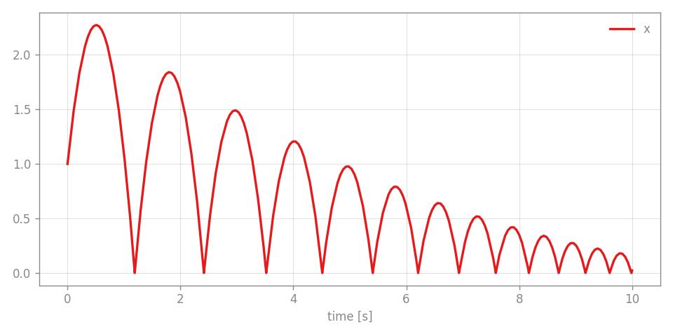

During the event handling, the simulator approaches the event until the specified tolerance is met. You can see this by analyzing the timesteps taken by the adaptive integrator RKBS32.

import numpy as np
import matplotlib.pyplot as plt

fig, ax = plt.subplots(figsize=(8,4), tight_layout=True, dpi=120)

time, _ = Sc.read()

#add detected events
for t in E1: ax.axvline(t, ls="--", c="k")

#plot the timesteps
ax.plot(time[:-1], np.diff(time))

ax.set_yscale("log")
ax.set_ylabel("dt [s]")
ax.set_xlabel("time [s]")
ax.grid(True)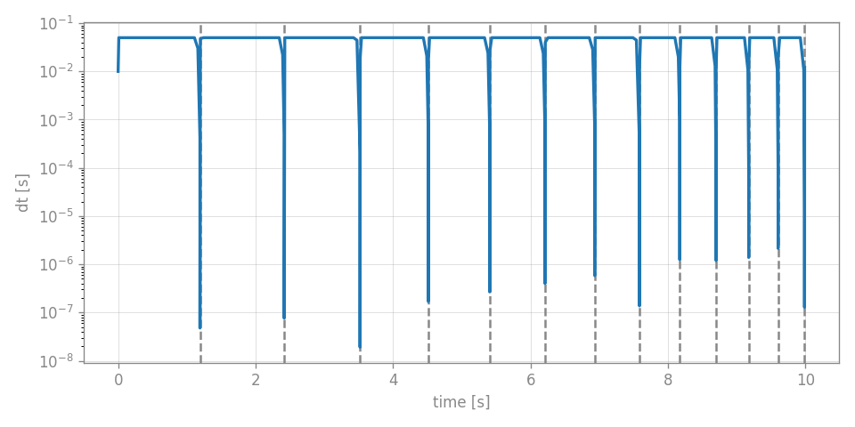

Contributing

PathSim is in active development and your feedback is highly appreciated! Dont shy away from filing issues or requests! If you want to contribute in a mayor way, send me a message and we can discuss how!