LinearRegression_Explained

This is a repository containing the explanation for Linear Regression using Sklearn, pandas, Numpy and Seaborn. Also performing Exploratory Data Analysis and Visualisation.
This explaination is divided into following parts and we will look each part in detail:

1. Understand the problem statement, dataset and choose ML model
2. Core Mathematics Concepts
3. Libraries Used
4. Explore the Dataset
5. Perform Visualisations
6. Perform Test_Train dataset split
7. Train the model
8. Perform the predictions
9. Model Metrics and Evaluations

1. Understand the problem Statement and the dataset

The data set is of the Housing price along with the various parameters affecting it. The target variable to be predicted is a set of continuous values; hence firming our choice to use the Linear Regeression model.

2. Core Mathematics Concepts

Tricks
Linear regression involves moving a line such that it is the best approximation for a set of points. The absolute trick and square trick are techniques to move a line closer to a point. Tricks are used for our understanding purposes.

i) Absolute Trick
A line with slope w1 and y-intercept w2 would have equation . To move the line closer to the point (p,q), the application of the absolute trick involves changing the equation of the line to where is the learning rate and is a small number whose sign depends on whether the point is above or below the line.

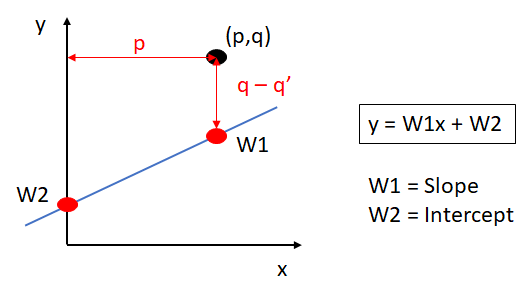
ii) Square Trick
A line with slope w1 and y-intercept w2 would have equation . The goal is to move the line closer to the point (p,q). A point on the line with the same y-coordinate as might be given by (p,q'). The distance between (p,q) and (p,q') is given by (q-q') . Following application of the square trick, the new equation would be given by where is the learning rate and is a small number whose sign does not depend on whether the point is above or below the line. This is due to the inclusion of the term that takes care of this implicitly.

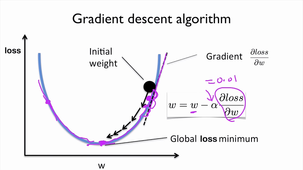
Gradient Descent (What actually happens in .fit())
It involves taking the derivative, or gradient, of the error function with respect to the weights, and taking a step in the direction of largest decrease.

The equation is as follows

Following several similar steps, the function will arrive at either a minimum or a value where the error is small. This is also referred to as “decreasing the error function by walking along the negative of its gradient".

3. Libraries Used

The following libraries are used intitally

import numpy as np
import pandas as pd
import seaborn as sns
import matplotlib.pyplot as plt

4. Explore the Dataset

We read the dataset into a Pandas dataframe

df=pd.read_csv('/content/housing.csv')

The .head() gives the first 5 rows along with all the columns info for a quick glimpse of dataset

df.head()

The .describe() function gives the description

df.describe()

The .info() function gives the quick infor on columns, type of data in them and valid entries

df.info()

5. Perform Visualisations

We use several function from seaborn library to visualize.
Seaborn is built on MatplotLib library with is built on MATLAB. So people experienced with MATLAB/OCTAVE will find its syntax similar.

Pairplot is quickly used to plot multiple pairwise bivariate distributions

sns.pairplot(df)

Heatmap gives a overview of how well different features are co-related

sns.heatmap(df.corr(), annot=True)

Jointplot gives visualizations with multiple pairwise plots with focus on a single relationship.

sns.jointplot(x='RM',y='MEDV',data=df)

Lmplot gives a Scatter plot with regression line

sns.lmplot(x='LSTAT', y='MEDV',data=df)
sns.lmplot(x='LSTAT', y='RM',data=df)

6. Perform Test_Train dataset split

We divide the Dataset into 2 parts, Train and test respectively.
We set test_size as 0.30 of dataset for validation. Random_state is used to ensure split is same everytime we execute the code

X_train,X_test,y_train,y_test=train_test_split(X,y,test_size=0.3,random_state=101)

7. Train the model

The mathematical concepts we saw above is implemented in single .fit() statement

from sklearn.linear_model import LinearRegression  #Importing the LinerRegression from sklearn
lm=LinearRegression()                              #Create LinerRegression object so the manupulation later is easy
lm.fit(X_train, y_train)                           #The fit happens here

8. Perform the predictions

Prediction of the values for testing set and save it in the predictions variable. The .coef_ module is used to get the coefficients(weights) that infuences the values of features

predictions=lm.predict(X_test)
lm.coef_

9. Model Metrics and Evaluations

The metrics are very important to inspect the accuracy of the model. The metrics are:

i) Mean Absolute Error (MAE) : It is the total sum of differences between predicted versus actual value divied by the number of points in dataset. Equation given by:

ii) Mean Squared Error (MSE) : It is the total of average squared difference between the estimated values and the actual values. Equation given by:

iii) Sqaure Root of Mean Sqare Error : Same as Mean Absolute Error, a good measure of accuracy, but only to compare prediction errors of different models or model configurations for a particular variable.

from sklearn import metrics
print(metrics.mean_absolute_error(y_test, predictions))
print(metrics.mean_squared_error(y_test, predictions))
print(np.sqrt(metrics.mean_squared_error(y_test, predictions)))