Version: 1.2.0 | Date: 2026-04-23 | Author: Valerio Lo Brano


pvfit5 estimates the five parameters of the single-diode model (SDM) of a photovoltaic module at Standard Test Conditions (STC: 1000 W/m² irradiance, 25 °C cell temperature) using only commercial datasheet values.
A genetic algorithm (DEAP) coupled with the CEC model implementation in pvlib minimises a weighted combination of relative errors on Voc, Isc, Vmp, and Imp — plus a stationarity constraint at the maximum power point — and reconstructs the full I–V curve via the Lambert W method.
Lo Brano, V. (2026). Open and Reproducible Estimation of PV Single-Diode Parameters from Datasheet Data. Energy Reports (Open Access, CC-BY).
DOI: 10.1016/j.egyr.2026.109280
A copy of the paper is included in this repository: paper/LoBrano2026_EnergyReports.pdf
See also CITATION.cff for machine-readable citation metadata.
If you use this software in your research, please cite the article above.
The single-diode model describes the I–V characteristic of a PV cell as:
I = I_L - I_0 [exp((V + I·R_s) / (n·N_s·V_th)) - 1] - (V + I·R_s) / R_sh
The five unknown parameters to be estimated are:
| Parameter | Symbol | Unit | Description |
|---|---|---|---|
| Photocurrent | I_L_ref |
A | Light-generated current at STC |
| Saturation current | I_o_ref |
A | Diode reverse saturation current at STC |
| Ideality factor | a_ref |
— | Modified diode ideality factor (n · N_s · V_th) |
| Series resistance | R_s |
Ω | Accounts for ohmic losses in contacts and bulk |
| Shunt resistance | R_sh |
Ω | Accounts for leakage current paths |
These parameters are estimated at STC (Standard Test Conditions):
- Irradiance: 1000 W/m²
- Cell temperature: 25 °C
The algorithm needs only the values that appear on a standard PV module datasheet at STC:
| Input | Symbol | Unit | Description |
|---|---|---|---|
| Open-circuit voltage | Voc | V | Voltage when no current flows |
| Short-circuit current | Isc | A | Current when terminals are short-circuited |
| Maximum power | Pmax | W | Maximum power at the MPP |
| Voltage at MPP | Vmp | V | Voltage at the maximum power point |
| Current at MPP | Imp | A | Current at the maximum power point |
Optional inputs (advanced users):
| Input | Unit | Default | Description |
|---|---|---|---|
| α_sc (alpha_sc) | A/°C | 0.05 | Short-circuit current temperature coefficient |
| EgRef | eV | 1.121 | Band gap energy at reference (crystalline Si) |
| dEgdT | eV/K | −0.000267 | Temperature coefficient of band gap |
The algorithm returns:
- The five SDM parameters (
I_L_ref,I_o_ref,a_ref,R_s,R_sh) at STC, which fully characterise the PV module. - Simulated key points (Voc, Isc, Vmp, Imp, Pmp from the fitted model) compared against the datasheet values.
- Total relative error — the weighted objective function value (lower is better), including individual errors on Voc, Isc, Vmp, Imp, and a stationarity residual at the maximum power point.
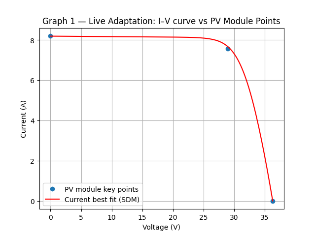
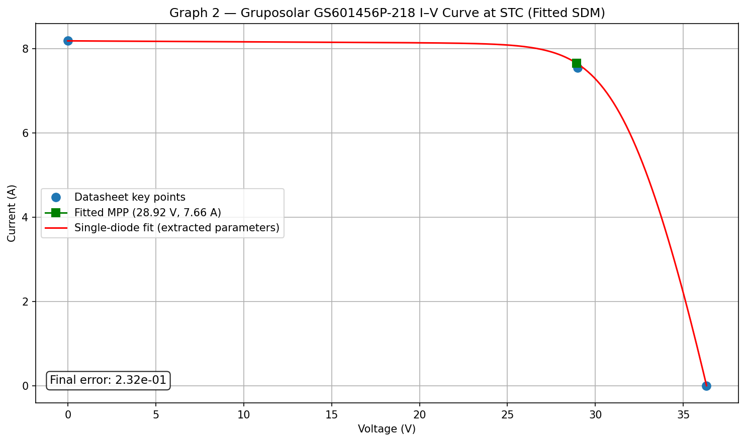
- I–V curve plot — a publication-quality figure showing the reconstructed curve with both the datasheet key points and the fitted maximum power point, so any discrepancy is immediately visible.
- Summary text file —
<MODULE_NAME>_CEC.txtwith all parameters and errors.
See example_output/Gruposolar_GS601456P-218.txt
for a complete text output example.
Graph 1 — Live adaptation (updates during GA evolution, auto-closes):
Graph 2 — Final I–V curve (publication-quality, stays open):
- Python ≥ 3.10
- pip
The following Python packages are required and are installed automatically by
pip install pvfit5:
| Package | Min version | Purpose |
|---|---|---|
| pvlib | 0.10 | CEC single-diode model and I–V solver (Lambert W) |
| DEAP | 1.4 | Genetic algorithm framework |
| NumPy | 1.24 | Numerical arrays |
| Matplotlib | 3.7 | Live and final I–V plots |
| SciPy | 1.10 | Statistical analysis |
| pandas | 2.0 | Dataframe handling and Excel I/O |
| openpyxl | 3.1 | Excel reading (.xlsx) |
| XlsxWriter | 3.1 | Excel writing (.xlsx) |
| seaborn | 0.12 | Statistical plots (batch analysis) |
| tqdm | 4.60 | Progress bar for the GA evolution |
From PyPI:
pip install pvfit5From GitHub (latest development version):
pip install git+https://github.com/valeriolobrano/pvfit5.gitFor local development (editable install):
git clone https://github.com/valeriolobrano/pvfit5.git
cd pvfit5
pip install -e .uv is a fast Python package manager that can replace pip and virtualenv.
Add to an existing project:
uv add pvfit5From GitHub:
uv add git+https://github.com/valeriolobrano/pvfit5.gitRun directly without installing (ephemeral):
uvx --from pvfit5 pvfit5 \
    --voc 36.3 --isc 8.19 --pmax 218.95 --vmp 29.0 --imp 7.55
Create a new project with pvfit5:
uv init my_pv_project
cd my_pv_project
uv add pvfit5
uv run pvfit5 --voc 36.3 --isc 8.19 --pmax 218.95 --vmp 29.0 --imp 7.55After installing pvfit5, run it from the terminal with your module datasheet values:
pvfit5 --voc 36.3 --isc 8.19 --pmax 218.95 --vmp 29.0 --imp 7.55All five datasheet values are required. Optional arguments:
| Argument | Description | Default |
|---|---|---|
--name |
Module name (for output files) | PVModule |
--error-target |
GA early-stop threshold | 1e-2 |
--alpha-sc |
α_sc in absolute units (A/°C) | 0.05 |
--alpha-sc-rel |
α_sc in relative units (1/°C); overrides --alpha-sc |
— |
--egref |
Band gap energy at reference conditions (eV) | 1.121 |
--degdt |
Temperature coefficient of band gap (eV/K) | -0.000267 |
--no-plot |
Disable live and final plots | — |
Full example:
pvfit5 --voc 36.3 --isc 8.19 --pmax 218.95 --vmp 29.0 --imp 7.55 \
--alpha-sc 0.05 --egref 1.121 --name MyModulefrom pvfit5.find_pv_parameters import fit_parameters, PVModuleData, STC, GAConfig
nd = PVModuleData(voc=36.3, isc=8.19, pmax=218.95, vmp=29.0, imp=7.55)
stc = STC() # default: EgRef=1.121, dEgdT=-0.000267
ga = GAConfig(error_target=1e-2)
results, summary = fit_parameters(nd, stc, ga, module_name="MyModule")
print(summary)
# Access individual results
print("R_s =", results["best_individual"]["R_s"], "Ω")
print("R_sh =", results["best_individual"]["R_sh"], "Ω")The script opens two plots:
- Graph 1 (live): I–V curve updating during GA evolution (auto-closes after 3 s).
- Graph 2 (final): publication-quality I–V curve with annotated errors
(stays open). Use
--no-plotto suppress both.
Run the algorithm on a large set of modules from the pvlib CEC database:
# Analyse 100 modules in alphabetical order
pvfit5-batch -n 100 --selection alpha

# Analyse 200 random modules (reproducible with --seed)
pvfit5-batch -n 200 --selection random --seed 42 --output my_results.xlsx
Results are saved to an Excel file. Run pvfit5-batch --help for all options.
After running pvfit5-batch, analyse the output Excel file:
# Analyse the default output file
pvfit5-analysis

# Analyse a specific file
pvfit5-analysis my_results.xlsx

# Suppress figure output
pvfit5-analysis my_results.xlsx --no-figures
The script produces:
- PDF and CDF plots for RMSE and runtime.
- Dominance analysis of partial errors.
results_summary.xlsxwith descriptive statistics.
For per-technology statistics:
pvfit5-parametric

# Or with a specific input and output file
pvfit5-parametric my_results.xlsx --output my_statistics.xlsxReleased under the BSD-3-Clause License. Free to use, modify, and redistribute, provided the original copyright notice is retained. The software is provided without warranty of any kind.